Lunar Frozen Orbits and Constellation Coverage

In this example, we will investigate the stability of Lunar Elliptical Frozen Orbits (ELFOs) over ten years and compute the surface coverage [1]. We will also demonstrate the capabilities of the open–source simulator LuPNT, developed by Stanford NAV Lab.

To run each cell, press Shift+Enter and wait for the code to execute. Most cells execute immediately, but some may take up to a minute to propagate satellite orbits. The output will be displayed below the cell, and you will automatically be directed to the next one.

This example consists of two parts. The first one is divided into six cases, where we explore how to propagate a spacecraft’s orbit with different levels of fidelity. Cases 2-6 are much shorter than Cases 1-2. In the second part, we look into the stability and coverage of a constellation with three satellites.

Please refer to the paper for additional details or insights into the results. If the propagation takes too long, please set recompute = False to use precomputed data.

Outline

• Part I: Building up

  • Case 0: Two-body propagation

  • Case 1: Three-body propagation (circular Moon orbit)

  • Case 2: Three-body propagation (JPL DE440 Ephemeris data)

  • Case 3: N-body propagation with Sun and 7x1 spherical harmonics

  • Case 4: Changing from inertial to rotating frame

  • Case 5: 50x50 spherical harmonics

  • Case 6: 10-year orbital propagation

• Part II: Coverage Analysis

  • Constellation stability

  • South pole coverage statistics

  • Entire surface coverage

References

[1] T. A. Ely, ‘Stable Constellations of Frozen Elliptical Inclined Lunar Orbits,’ J of Astronaut Sci, vol. 53, no. 3, pp. 301–316, Sep. 2005, doi: 10.1007/BF03546355.

Part I: Building up

# **************************
import pylupnt as pnt
# **************************

import numpy as np
import matplotlib
import plotly.graph_objects as go
import matplotlib.pyplot as plt
from ex_frozen_orbits.ex_frozen_orbits_utils import *

Found required data at ../../../LuPNT_data

Case 0

In this first case, we propagate the satellite orbit using two-body dynamics to familiarize ourselves with the type of orbit and the simulator’s capabilities. We start by defining the propagation start and end times and the time for which we want to store the satellite position and velocity.

As in [1], we will set the starting epoch as 15 July 2009 at 1:00:00. Our simulator uses a time scale called International Atomic Time (TAI) to propagate spacecraft orbits. This time is closely related to Ephemeris Time (ET), Barycentric Dynamical Time (TDB), and Atomic Time (A.1), which are used in tools like NASA’s CSPICE and GMAT.

# International Atomic Time (TAI)
t0 = pnt.gregorian2time(2009, 7, 15, 1, 0, 0)  # [s]

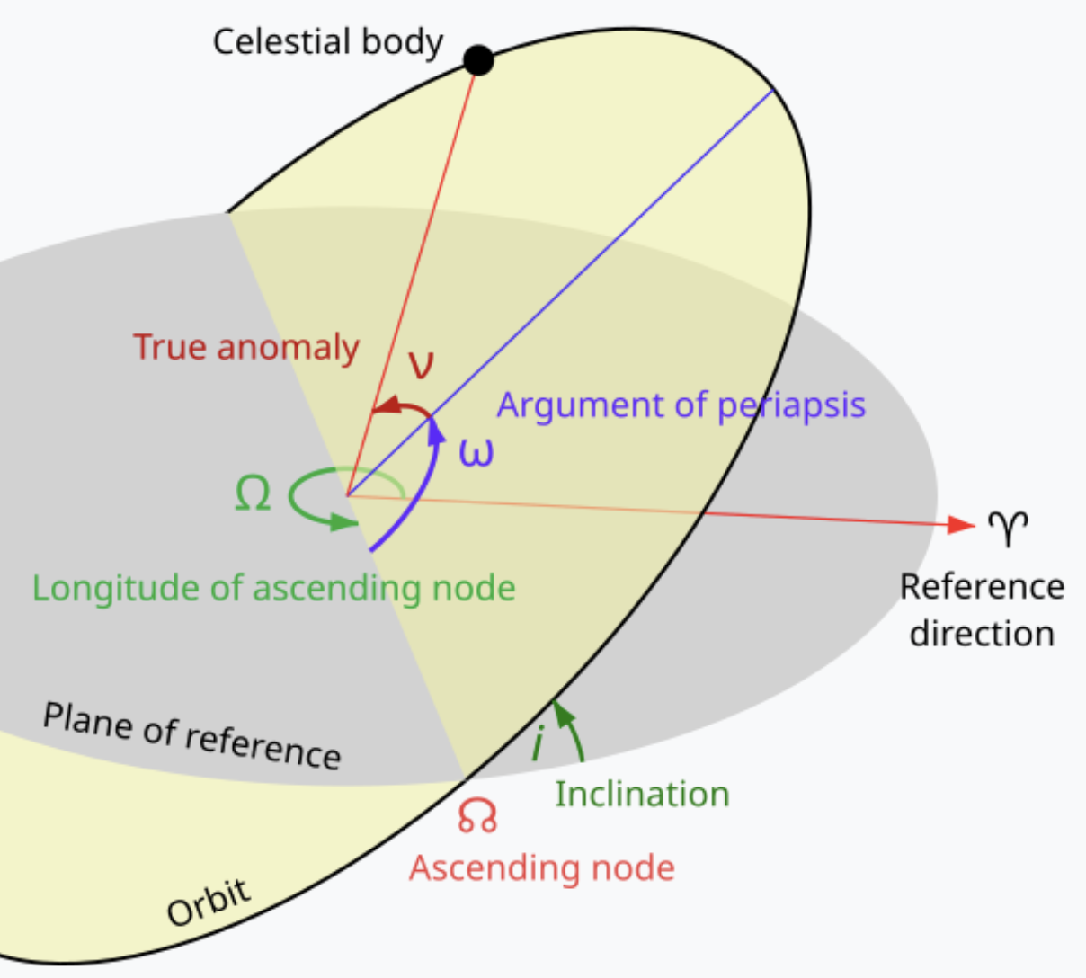
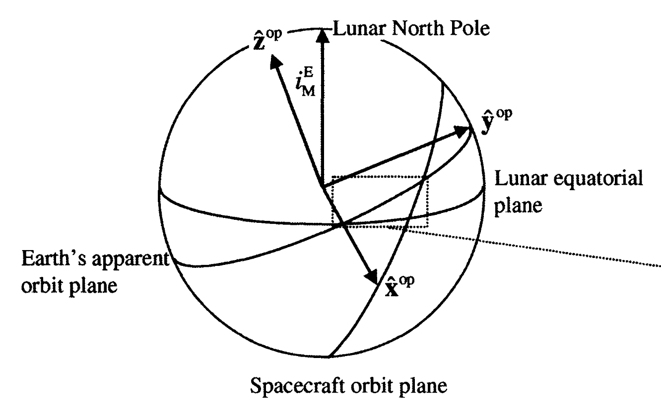
To verify the stability of ELFOs, we will propagate a satellite in lunar orbit. We define its orbital elements in the Orbital Plane (OP) frame, a reference frame centered at the Moon that is rotated to match the apparent orbit of the Earth around the Moon. This frame proves useful for analytically studying Earth’s gravitational perturbations on a lunar satellite. We observe that the satellite has an orbital period of approximately 13 hours.

# Classical Orbital Elements (COE)
a = 6541.4  # [km] Semi-major axis
e = 0.6000  # [--] Eccentricity
i = 56.2 * pnt.RAD  # [deg] Inclination
O = 0.00 * pnt.RAD  # [deg] Right ascension of the ascending node
w = 90.0 * pnt.RAD  # [deg] Argument of perigee
M = 0.00 * pnt.RAD  # [deg] Mean anomaly

coe0_op = np.array([a, e, i, O, w, M])

sat_period = pnt.get_orbital_period(a, pnt.GM_MOON)  # [s] Satellite period
print(f"Satellite period {sat_period / pnt.SECS_HOUR:.2f} h")

Satellite period 13.19 h

Let’s propagate the satellite position and velocity during one orbit. We start by defining the duration of the propagation as well as the propagation time step.

# Time
dt_total_1orb = sat_period  # [s] Total duration
dt_step_1orb = 5 * pnt.SECS_MINUTE  # [s] Time step
dt_prop_1orb = 20  # [s] Propagation time step

tspan_1orb = np.arange(0, dt_total_1orb + dt_step_1orb, dt_step_1orb)  # [s] Time span
tfs_1orb = t0 + tspan_1orb  # [s] Time in TAI
n_steps_1orb = len(tspan_1orb)

print(f"Total duration    {dt_total_1orb/pnt.SECS_DAY:.2f} days")
print(f"Time step         {dt_step_1orb/pnt.SECS_MINUTE:.2f} minutes")
print(f"Propagation step  {dt_prop_1orb} seconds")
print(f"Start epoch       {pnt.time2gregorian_string(t0)} TAI")
print(f"End epoch         {pnt.time2gregorian_string(tfs_1orb[-1])} TAI")
print(f"Number of steps   {n_steps_1orb}")

Total duration    0.55 days
Time step         5.00 minutes
Propagation step  20 seconds
Start epoch       2009/07/15 01:00:00.000 TAI
End epoch         2009/07/15 14:15:00.000 TAI
Number of steps   160

To propagate a spacecraft, we can use different dynamics models, ranging from those based on orbital elements, which usually provide analytical expressions, to numerically integrating differential equations that include different perturbations. We typically want to use the most complete models to propagate ground truth orbits. When performing Orbit Determination, we want to use the simplest model that meets the mission navigation requirements.

We will propagate the satellite orbit using two-body dynamics in this first example. We will numerically propagate the satellite’s position and velocity using the Moon’s gravitational perturbation. We compute the acceleration due to the Moon’s gravity and integrate the equations of motion using a 4th-order Runge-Kutta integrator.

Below is an example of how to set up this dynamics model, convert the initial orbital elements to initial position and velocity, and propagate the satellite orbit–everything in the OP frame.

# Dynamics
dyn_2body = pnt.CartesianTwoBodyDynamics(pnt.GM_MOON)  # Keplerian dynamics
dyn_2body.set_time_step(dt_prop_1orb)  # Propagation time step

# Initial conditions
rv0_op = pnt.classical2cart(coe0_op, pnt.GM_MOON)  # [km, km/s] Position and velocity

# Propagte
rv_case0_op = dyn_2body.propagate(rv0_op, t0, tfs_1orb)  # Propagated orbital elements

print(f"Initial orbital elements       {coe0_op} [km, rad]")
print(f"Initial position and velocity  {rv0_op} [km, km/s]")
print(f"Shape of rv_case0_op           {rv_case0_op.shape}")

Initial orbital elements       [6541.4       0.6       0.9809    0.        1.5708    0.    ] [km, rad]
Initial position and velocity  [   0.     1455.5809 2174.3207   -1.7315    0.        0.    ] [km, km/s]
Shape of rv_case0_op           (160, 6)

We can easily visualize the orbit using LuPNT’s plotting functions. The 3D plot should be interactive, so feel free to move it around to get a better perspective.

# Plot
fig = go.Figure()
pnt.plot.plot_body(fig, pnt.MOON)
pnt.plot.plot_orbits(fig, rv_case0_op, t=0)
pnt.plot.set_view(fig, azimuth=-35, elevation=10, zoom=3)
fig.add_annotation(
    text=case0_0_text.format(dt_total_1orb / pnt.SECS_HOUR), **case0_0_text_args
)
fig.update_layout(width=400, height=400)
fig.show()

Case 1

Let’s move away from the previous simplified example and explore LuPNT’s flexibility by implementing a two-year propagation with Earth as the only perturbation. Still working on the OP frame, we will assume that the Moon’s orbit around the Earth, and thus the Earth’s apparent motion around the Moon, is perfectly circular. This case illustrates the basic motions predicted by simplified analytical expressions presented in the paper [1].

As in the previous case, let’s define the propagation times. Recall that the Moon’s orbital period is approximately 27 days.

# Time
dt_total_2yr = 2 * pnt.DAYS_YEAR * pnt.SECS_DAY  # [s] Total duration
dt_step_2yr = 60 * pnt.SECS_MINUTE  # [s] Time step
dt_prop_2yr = 1 * pnt.SECS_MINUTE  # [s] Propagation step

tspan_2yr = np.arange(0, dt_total_2yr + dt_step_2yr, dt_step_2yr)  # [s] Time span
tfs_2yr = t0 + tspan_2yr  # [s] Time in TAI
n_steps_2yr = len(tspan_2yr)

print(f"Total duration    {dt_total_2yr/pnt.SECS_DAY:.2f} days")
print(f"Time step         {dt_step_2yr/pnt.SECS_MINUTE:.2f} minutes")
print(f"Propagation step  {dt_prop_2yr} seconds")
print(f"Start epoch       {pnt.time2gregorian_string(t0)} TAI")
print(f"End epoch         {pnt.time2gregorian_string(tfs_2yr[-1])} TAI")
print(f"Number of steps   {n_steps_2yr}")

moon_period = pnt.get_orbital_period(pnt.D_EARTH_MOON, pnt.GM_EARTH)
print(f"\nMoon period: {moon_period / pnt.SECS_DAY:.3f} days")

Total duration    730.50 days
Time step         60.00 minutes
Propagation step  60.0 seconds
Start epoch       2009/07/15 01:00:00.000 TAI
End epoch         2011/07/15 13:00:00.000 TAI
Number of steps   17533

Moon period: 27.452 days

Now, let’s propagate the Moon’s position and velocity around the Earth. Instead of numerically propagating the Moon’s position and velocity using the Earth’s gravitational perturbation, we will use analytical Keplerian dynamics to propagate its orbital elements. We will use the JPL DE440 ephemeris data to find the Moon’s initial position and velocity and convert it to orbital elements. The Moon’s orbit around Earth in the OP frame approximately lies in the x-y plane, which is not the case for other inertial reference frames.

# Dynamics
dyn_moon = pnt.KeplerianDynamics(pnt.GM_EARTH)

# Initial conditions
rv0_moon_op = pnt.get_body_pos_vel(t0, pnt.EARTH, pnt.MOON, pnt.MOON_OP)
coe0_moon_op = pnt.cart2classical(rv0_moon_op, pnt.GM_EARTH)

# Propagate
coe_moon_op = dyn_moon.propagate(coe0_moon_op, t0, tfs_2yr)

# Convert
rv_moon_op = pnt.classical2cart(coe_moon_op, pnt.GM_EARTH)

# Plot
fig = go.Figure()
pnt.plot.plot_body(fig, pnt.EARTH)
pnt.plot.plot_orbits(fig, rv_moon_op, t=0)
pnt.plot.set_view(fig, azimuth=-130, elevation=25, zoom=8)
fig.add_annotation(
    text=case1_0_text.format(dt_total_2yr / pnt.SECS_DAY), **case1_0_text_args
)
fig.update_layout(width=400, height=400)
fig.show()

Now that we have the Moon’s position, we can modify the dynamics to propagate the satellite’s orbit around the Moon to introduce Earth’s gravitational perturbation. The simulator includes dynamics with multiple celestial bodies. Still, this example illustrates how we can work with different assumptions like perfectly circular orbit or use custom dynamics models for applications like Orbit Determination.

Below, we extend a two-body dynamics class to include Earth’s gravitational acceleration.

class MyDynamicsWithEarth(pnt.CartesianTwoBodyDynamics):

    def __init__(self, GM):
        super().__init__(GM)  # Initialize CartesianTwoBodyDynamics
        self.GM = GM  # Store the gravitational parameter
        self.set_ode_function(self.compute_rates)  # Set the differential equation

    def compute_rates(self, t, rv):
        # Earth position and velocity
        coe_moon_op = dyn_moon.propagate(coe0_moon_op, t0, t)
        rv_earth_op = -pnt.classical2cart(coe_moon_op, pnt.GM_EARTH)

        # Moon acceleration
        rv_dot_op = super().compute_rates(t, rv)

        # Earth acceleration
        rv_dot_op[3:] += pnt.acceleration_point_mass(
            rv[:3], rv_earth_op[:3], pnt.GM_EARTH
        )

        return rv_dot_op

With our new dynamics model, let’s now propagate the satellite orbit around the Moon for two years.

# Propagate
recompute = False

dyn_3body_circ = MyDynamicsWithEarth(pnt.GM_MOON)
dyn_3body_circ.set_time_step(dt_prop_2yr)

if recompute or not data_part1_exists:
    rv_case1_op = dyn_3body_circ.propagate(rv0_op, t0, tfs_2yr, progress=True)
else:
    with pnt.File(data_part1_path, "r") as f:
        rv_case1_op = np.array(f["rv_case1_op"])

/var/folders/m9/t0lwgrj15w37pjv7jdy9m0g40000gp/T/ipykernel_21061/753579617.py:11: DeprecationWarning:

__array__ implementation doesn't accept a copy keyword, so passing copy=False failed. __array__ must implement 'dtype' and 'copy' keyword arguments.

Earth’s gravitational perturbation can cause instability in the satellite’s orbit. However, the orbit we defined in the previous case remains stable under the earlier assumptions. Let’s plot a few of the satellite’s revolutions over the past two years to see how orbit evolves.

# Plot
n_plot = 20
tspan_plot = np.arange(0, sat_period, dt_prop_2yr)
rv_plot_op = np.zeros((n_plot, len(tspan_plot), 6))
for i in range(n_plot):
    j = int(i * n_steps_2yr / n_plot)
    rv_plot_op[i] = dyn_3body_circ.propagate(
        rv_case1_op[j], tfs_2yr[j], tfs_2yr[j] + tspan_plot
    )

fig = go.Figure()
pnt.plot.plot_body(fig, pnt.MOON)
pnt.plot.plot_orbits(
    fig,
    rv_plot_op,
    color=pnt.plot.sample_colorscale("Blues", np.linspace(0, 1, n_plot)),
)
pnt.plot.set_view(fig, azimuth=-130, elevation=10, zoom=2.5)
fig.add_annotation(
    text=case1_1_text.format(dt_total_2yr / pnt.SECS_DAY), **case1_1_text_args
)
fig.update_layout(width=400, height=400)
fig.show()

We can visualize the evolution of the satellite’s orbit by plotting its orbital elements over time. We can see how the rotation of the orbit in the secular drift of the right ascension of the ascending node. We see that the eccentricity, inclination, and argument of periapsis have long-term and short-term osculations but remain bounded.

# Plot
coe_case1_op = pnt.cart2classical(rv_case1_op, pnt.GM_MOON)
labels = [
    "Semi-major axis [km]",
    "Eccentricity [-]",
    "Inclination [deg]",
    "Right Asc. [deg]",
    "Arg. of Periapsis [deg]",
    "Mean Anomaly [deg]",
]

fig = plt.figure(figsize=(8, 6))
matplotlib.rcParams.update({"font.size": 12})
x = tspan_2yr / pnt.SECS_DAY
plt.suptitle("Orbital Elements")
for i in range(6):
    plt.subplot(3, 2, i + 1)
    y = coe_case1_op[:, i] if i < 2 else coe_case1_op[:, i] * pnt.DEG
    plt.plot(x, y)
    plt.xlabel("Days past " + pnt.time2gregorian_string(t0) + " TAI")
    plt.ylabel(labels[i])
    plt.grid()
    if i < 5:
        plt.xlim(x[0], x[-1])
    else:
        plt.xlim(x[0], x[100])
plt.tight_layout()
plt.show()

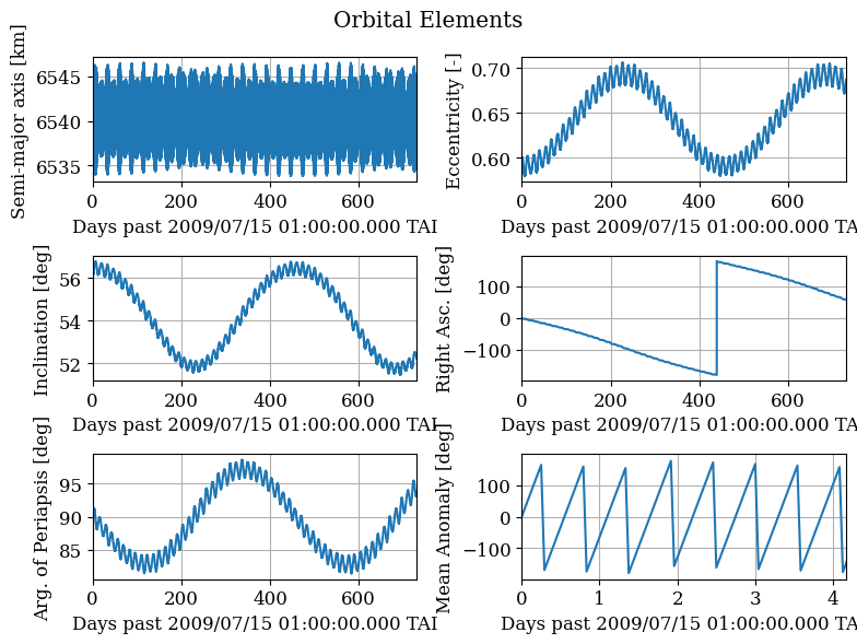
With the addition of the Earth’s gravitational perturbation, even with a perfectly circular orbit, the evolution of the satellite’s orbit becomes complex. In the following cases, we will add more perturbations to the dynamics model to better understand the stability of the satellite’s orbit and compare them at the end.

Case 2

This case is the same as Case 1, except now the true ephemeris for the Earth is used (JPL DE440). This case examines the impact of introducing eccentricity to the Moon’s orbit around the Earth. For this, we will use LuPNT’s n-body dynamics class, which can include multiple celestial bodies and gravity models, as well as other perturbations like solar radiation pressure or atmospheric drag.

# Dynamics
dyn_3body = pnt.NBodyDynamics(pnt.IntegratorType.RK4)
dyn_3body.add_body(pnt.Body.Moon())
dyn_3body.add_body(pnt.Body.Earth())
dyn_3body.set_time_step(dt_prop_2yr)
dyn_3body.set_frame(pnt.MOON_CI)

# Propagate
recompute = False

rv0_ci = pnt.convert_frame(t0, rv0_op, pnt.MOON_OP, pnt.MOON_CI)
if recompute or not data_part1_exists:
    rv_case2_ci = dyn_3body.propagate(rv0_ci, t0, tfs_2yr[:, None], True)
else:
    with pnt.File(data_part1_path, "r") as f:
        rv_case2_ci = np.array(f["rv_case2_mi"])

/var/folders/m9/t0lwgrj15w37pjv7jdy9m0g40000gp/T/ipykernel_21061/3108274925.py:9: DeprecationWarning:

__array__ implementation doesn't accept a copy keyword, so passing copy=False failed. __array__ must implement 'dtype' and 'copy' keyword arguments.

# Convert
rv_case2_op = pnt.convert_frame(tfs_2yr, rv_case2_ci, pnt.MOON_CI, pnt.MOON_OP)
coe_case2_op = pnt.cart2classical(rv_case2_op, pnt.GM_MOON)

Case 3

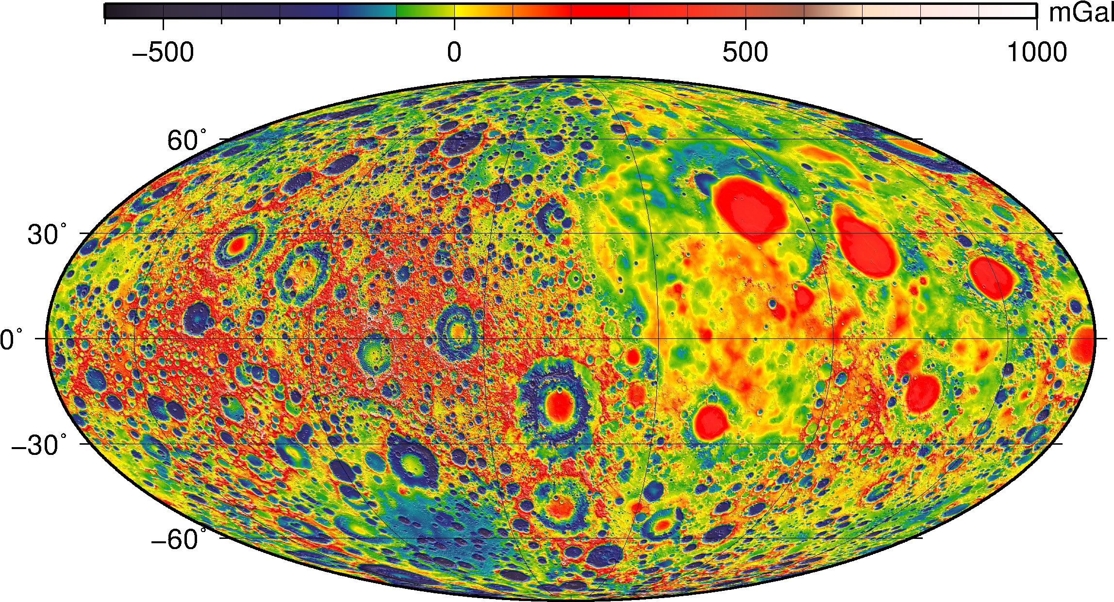
The same as Case 2, except now perturbations from the Earth, Sun, and zonal harmonics through \(J_7\) are included. This case examines the impact of introducing additional gravity terms.

# Dynamics
dyn_nbody = pnt.NBodyDynamics(pnt.IntegratorType.RK4)
dyn_nbody.add_body(pnt.Body.Moon(7, 1))
dyn_nbody.add_body(pnt.Body.Earth())
dyn_nbody.add_body(pnt.Body.Sun())
dyn_nbody.set_time_step(dt_prop_2yr)
dyn_nbody.set_frame(pnt.MOON_CI)

# Propagate
recompute = False

if recompute or not data_part1_exists:
    rv_case3_ci = dyn_nbody.propagate(rv0_ci, t0, tfs_2yr, progress=True)
else:
    with pnt.File(data_part1_path, "r") as f:
        rv_case3_ci = np.array(f["rv_case3_mi"])

/var/folders/m9/t0lwgrj15w37pjv7jdy9m0g40000gp/T/ipykernel_21061/1149665572.py:8: DeprecationWarning:

__array__ implementation doesn't accept a copy keyword, so passing copy=False failed. __array__ must implement 'dtype' and 'copy' keyword arguments.

# Convert
rv_case3_op = pnt.convert_frame(tfs_2yr, rv_case3_ci, pnt.MOON_CI, pnt.MOON_OP)
coe_case3_op = pnt.cart2classical(rv_case3_op, pnt.GM_MOON)

Case 4

The same as Case 3, except now we observe the evolution of the orbital elements in the mean-Earth/polar (ME) frame (also known as IAU Moon Pole). This case examines the effect of switching from a frame aligned with Earth’s orbital plane to one aligned with the Moon’s equatorial plane. We only need to convert the satellite’s position and velocity to this new frame.

# Convert
rv_case4_me = pnt.convert_frame(
    tfs_2yr, rv_case3_ci, pnt.MOON_CI, pnt.MOON_ME, rotate_only=True
)
coe_case4_me = pnt.cart2classical(rv_case4_me, pnt.GM_MOON)

Case 5

The same as Case 4, except now a complete 50x50 lunar gravity field is used. This case examines the effect of the additional zonal and tesseral harmonics on the evolution of the trajectory.

# Dynamics
dyn_nbody50 = pnt.NBodyDynamics(pnt.IntegratorType.RK4)
dyn_nbody50.add_body(pnt.Body.Moon(50, 50))
dyn_nbody50.add_body(pnt.Body.Earth())
dyn_nbody50.add_body(pnt.Body.Sun())
dyn_nbody50.set_time_step(dt_prop_2yr)
dyn_nbody50.set_frame(pnt.MOON_CI)

# Propagate
recompute = False

if recompute or not data_part1_exists:
    rv_case5_ci = dyn_nbody50.propagate(rv0_ci, t0, tfs_2yr, progress=True)
else:
    with pnt.File(data_part1_path, "r") as f:
        rv_case5_ci = np.array(f["rv_case5_mi"])

/var/folders/m9/t0lwgrj15w37pjv7jdy9m0g40000gp/T/ipykernel_21061/3845413523.py:8: DeprecationWarning:

__array__ implementation doesn't accept a copy keyword, so passing copy=False failed. __array__ must implement 'dtype' and 'copy' keyword arguments.

# Convert
rv_case5_me = pnt.convert_frame(
    tfs_2yr, rv_case5_ci, pnt.MOON_CI, pnt.MOON_ME, rotate_only=True
)
coe_case5_me = pnt.cart2classical(rv_case5_me, pnt.GM_MOON)

Case 6

The same as Case 4, except now the propagation interval is ten years. This case illustrates the long-term stability of the orbit and later will be used to demonstrate the coverage properties of the entire constellation.

# Time
dt_total_10yr = 10 * pnt.DAYS_YEAR * pnt.SECS_DAY  # [s] Total duration
dt_step_10yr = 60.0 * pnt.SECS_MINUTE  # [s] Time step
dt_prop_10yr = 1.0 * pnt.SECS_MINUTE  # [s] Propagation step

tspan_10yr = np.arange(0, dt_total_10yr + dt_step_10yr, dt_step_10yr)  # [s] Time span
tfs_10yr = t0 + tspan_10yr  # [s] Time in TAI
n_steps_10yr = len(tspan_10yr)

print(f"Total duration    {dt_total_10yr/pnt.SECS_DAY/pnt.DAYS_YEAR:.2f} years")
print(f"Time step         {dt_step_10yr/pnt.SECS_MINUTE:.2f} minutes")
print(f"Propagation step  {dt_prop_10yr} seconds")
print(f"Start epoch       {pnt.time2gregorian_string(t0)} TAI")
print(f"End epoch         {pnt.time2gregorian_string(tfs_10yr[-1])} TAI")
print(f"Number of steps   {n_steps_10yr}")

Total duration    10.00 years
Time step         60.00 minutes
Propagation step  60.0 seconds
Start epoch       2009/07/15 01:00:00.000 TAI
End epoch         2019/07/15 13:00:00.000 TAI
Number of steps   87661

# Propagate
recompute = False

if recompute or not data_part1_exists:
    rv_case6_ci = dyn_nbody.propagate(rv0_ci, t0, tfs_10yr, progress=True)
else:
    with pnt.File(data_part1_path, "r") as f:
        rv_case6_ci = np.array(f["rv_case6_mi"])

/var/folders/m9/t0lwgrj15w37pjv7jdy9m0g40000gp/T/ipykernel_21061/2857897023.py:8: DeprecationWarning:

__array__ implementation doesn't accept a copy keyword, so passing copy=False failed. __array__ must implement 'dtype' and 'copy' keyword arguments.

# Convert
rv_case6_me = pnt.convert_frame(
    tfs_10yr, rv_case6_ci, pnt.MOON_CI, pnt.MOON_ME, rotate_only=True
)
coe_case6_me = pnt.cart2classical(rv_case6_me, pnt.GM_MOON)

Orbital Elements

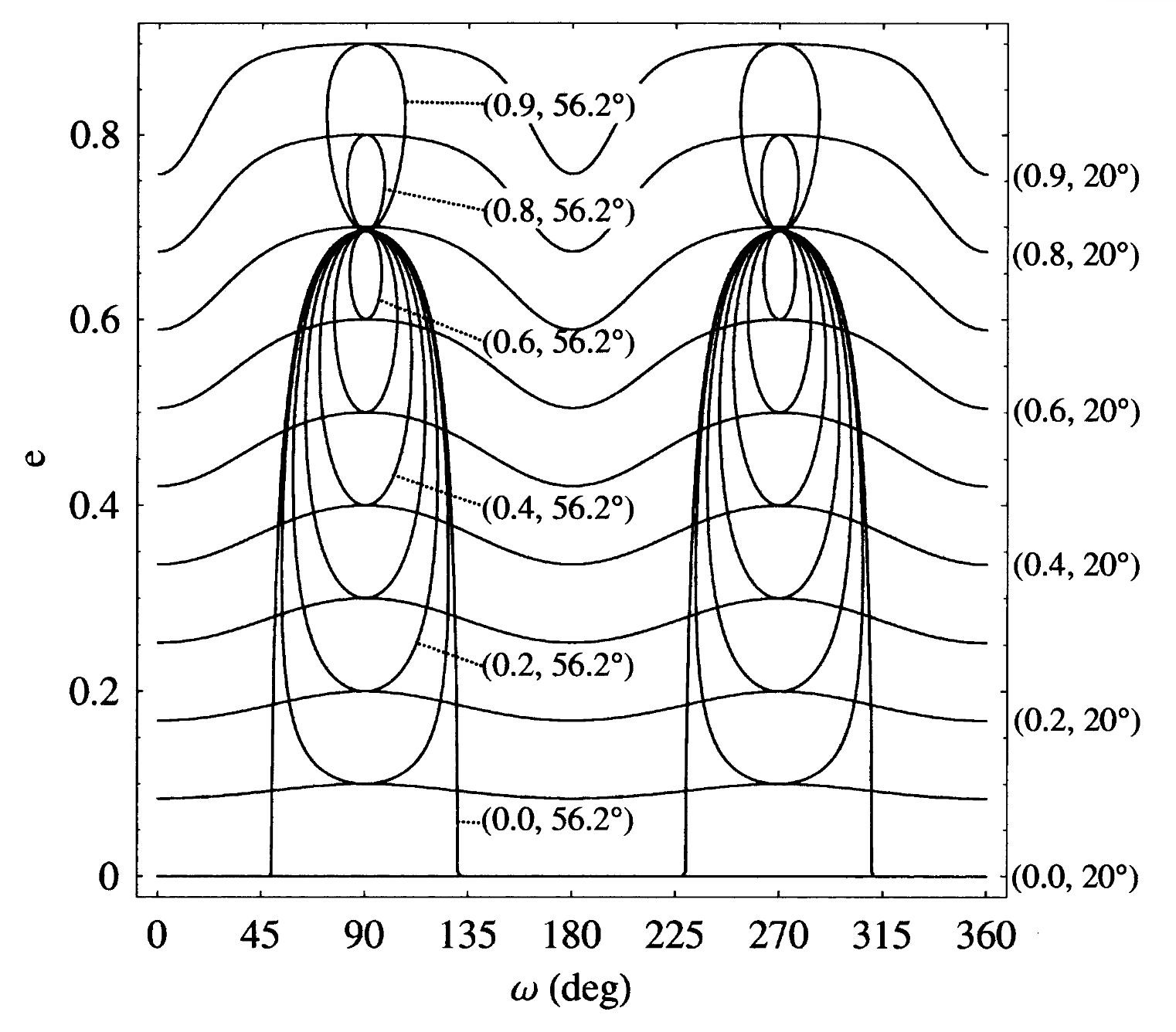
The stability of a satellite’s orbit can be analyzed by studying the phase plane formed by the eccentricity and argument of periapsis (e-w plane). The paper explores which orbits are stable by finding the evolution of the satellite’s orbit in the e-w plane. Let’s plot the e-w planes for the 6 cases. The figure below shows that orbits with \(\omega=90^\circ\) and \(\omega=270^\circ\) can be stable.

# Plot
coe_cases = [
    coe_case1_op,
    coe_case2_op,
    coe_case3_op,
    coe_case4_me,
    coe_case5_me,
    coe_case6_me,
]
titles = [
    "Case 1: Circ Earth Orbit, OP Frame",
    "Case 2: DE440 Eph, Earth, OP Frame",
    "Case 3: DE440 Eph, Earth, Sun, 7x1 grav, OP Frame",
    "Case 4: DE440 Eph, Earth, Sun, 7x1 grav, ME Frame",
    "Case 5: DE440 Eph, Earth, Sun, 50x50 grav, ME Frame",
    "Case 6: 10 year Propagation of Case 4",
]

fig = plt.figure(figsize=(8, 8))
matplotlib.rcParams.update({"font.size": 10})
plt.suptitle("e - w Phase Plane Plots for the Six Cases.")

for i, coe in enumerate(coe_cases):
    plt.subplot(3, 2, i + 1)
    plt.plot(coe[:, 4] * pnt.DEG, coe[:, 1], lw=1)
    plt.xlabel("Arg. of periapsis [deg]")
    plt.ylabel("Eccentricity [-]")
    plt.title(titles[i], fontsize=10)
    plt.grid()
    plt.xlim(70, 110)
    plt.ylim(0.50, 0.75)

plt.tight_layout()
plt.show()

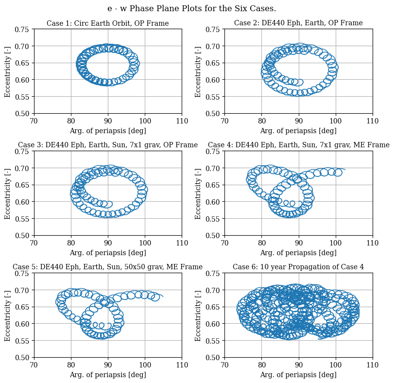
The paper offers detailed insights to these results but the key takeaways are: - The addition of the true ephemeris in Case 2 increases the size of the libration. - In Case 3 the addition of Sun gravity and zonal gravity in Case 3 do not significantly affect the motion over Case 2. - In Cases 4,5, and 6 the frame has changed to ME (IAU Moon Pole) and the libration increases in complexity by adding some long period loops, however the motion is still bounded and the amplitude of the eccentricity variation remains about the same as in Cases 2 and 3. - The addition of the complete 50x50 field had no significant impact on the overall results.

Finally, the orbit presents long-term stability, indicating that it is amenable to constellation design.

Part II: Coverage Analysis

Constellation stability

The paper presents a method to design a constellation with three satellites such that each satellite sees the South Pole during every orbital revolution over a ten-year mission. Because of the complexity of the motion, it is nearly impossible to ascertain the coverage and stability of the design analytically. Via numerical simulation, however, it is possible to find a design that provides stable two-fold coverage of the South Pole, i.e., two satellites are always visible from the South Pole.

Let’s start by propagating the orbits of the three satellites and see the evolution of their orbital elements over time. We will use the same dynamics model as in Case 6.

# Classical Orbital Elements (COE)
n_sat = 3
coes0_op = np.array(
    [
        [6541.4, 0.6, 56.2 * pnt.RAD, 0, 90 * pnt.RAD, 0],
        [6541.4, 0.6, 56.2 * pnt.RAD, 0, 90 * pnt.RAD, 120 * pnt.RAD],
        [6541.4, 0.6, 56.2 * pnt.RAD, 0, 90 * pnt.RAD, 240 * pnt.RAD],
    ]
)

# Time
dt_total_cov = 2 * pnt.DAYS_YEAR * pnt.SECS_DAY  # [s] Total duration
dt_step_cov = 15 * pnt.SECS_MINUTE  # [s] Time step
dt_prop_cov = 60  # [s] Propagation step

tspan_cov = np.arange(0, dt_total_cov + dt_step_cov, dt_step_cov)  # [s] Time span
tfs_cov = t0 + tspan_cov  # [s] Time in TAI
n_steps_cov = len(tspan_cov)

print(f"Total duration    {dt_total_cov/pnt.SECS_DAY:.2f} days")
print(f"Time step         {dt_step_cov/pnt.SECS_MINUTE:.2f} minutes")
print(f"Propagation step  {dt_prop_cov} seconds")
print(f"Start epoch       {pnt.time2gregorian_string(t0)} TAI")
print(f"End epoch         {pnt.time2gregorian_string(tfs_cov[-1])} TAI")
print(f"Number of steps   {n_steps_cov}")

Total duration    730.50 days
Time step         15.00 minutes
Propagation step  60 seconds
Start epoch       2009/07/15 01:00:00.000 TAI
End epoch         2011/07/15 13:00:00.000 TAI
Number of steps   70129

# Propagate
recompute = False
rvs_ci = np.zeros((n_sat, n_steps_cov, 6))

if recompute or not data_part2_exists:
    for i in range(3):
        rv0_op_i = pnt.classical2cart(coes0_op[i], pnt.GM_MOON)
        rv0_mi_i = pnt.convert_frame(t0, rv0_op_i, pnt.MOON_OP, pnt.MOON_CI)
        rvs_ci[i] = dyn_nbody.propagate(rv0_mi_i, t0, tfs_cov, progress=True)
else:
    with pnt.File(data_part2_path, "r") as f:
        for i in range(3):
            rvs_ci[i] = np.array(f[f"rvs_mi{i}"])

/var/folders/m9/t0lwgrj15w37pjv7jdy9m0g40000gp/T/ipykernel_21061/1549470208.py:13: DeprecationWarning:

__array__ implementation doesn't accept a copy keyword, so passing copy=False failed. __array__ must implement 'dtype' and 'copy' keyword arguments.

# Plot
plot_mean_anomaly_differences(tfs_cov, rvs_ci, set_lims=False)

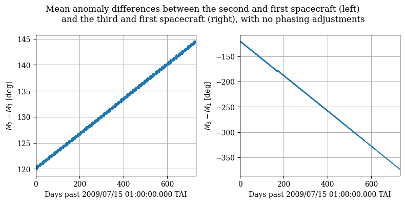
While the orbits are stable, there is a drift between the relative positions of the satellites, which can lead to a loss of coverage. For example, on the right plot, we observe that the difference in mean anomaly will pass -360 degrees, i.e., 0 degrees.

To ensure that the satellites maintain the desired coverage, we need to adjust the initial conditions of the orbits. The paper presents a numerical method to find differences in the semi-major axis such that the secular drift in the mean anomaly is compensated.

Constellation stability (Phasing Adjusted)

Let’s propagate again, updating the semi-major axis of the spacecraft to be - \(a_1 = 6541.4\) km - \(a_2 = 6541.623458\) km - \(a_3 = 6539.069348\) km

# Classical Orbital Elements (COE)
n_sat = 3
coes0_op_adjusted = np.array(
    [
        [6541.400000, 0.6, 56.2 * pnt.RAD, 0, 90 * pnt.RAD, 0],
        [6541.623458, 0.6, 56.2 * pnt.RAD, 0, 90 * pnt.RAD, 120 * pnt.RAD],
        [6539.069348, 0.6, 56.2 * pnt.RAD, 0, 90 * pnt.RAD, 240 * pnt.RAD],
    ]
)

# Propagate
recompute = False
rvs_mi_adjusted = np.zeros_like(rvs_ci)

if recompute or not data_part2_exists:
    for i in range(3):
        rv0_op_i = pnt.classical2cart(coes0_op_adjusted[i], pnt.GM_MOON)
        rv0_mi_i = pnt.convert_frame(t0, rv0_op_i, pnt.MOON_OP, pnt.MOON_CI)
        rvs_mi_adjusted[i] = dyn_nbody.propagate(rv0_mi_i, t0, tfs_cov, progress=True)
else:
    with pnt.File(data_part2_path, "r") as f:
        for i in range(3):
            rvs_mi_adjusted[i] = np.array(f[f"rvs_mi_adjusted{i}"])
    print("Loaded from file")

Loaded from file

/var/folders/m9/t0lwgrj15w37pjv7jdy9m0g40000gp/T/ipykernel_21061/22196204.py:13: DeprecationWarning:

__array__ implementation doesn't accept a copy keyword, so passing copy=False failed. __array__ must implement 'dtype' and 'copy' keyword arguments.

# Plot
plot_mean_anomaly_differences(tfs_cov, rvs_mi_adjusted, set_lims=True)

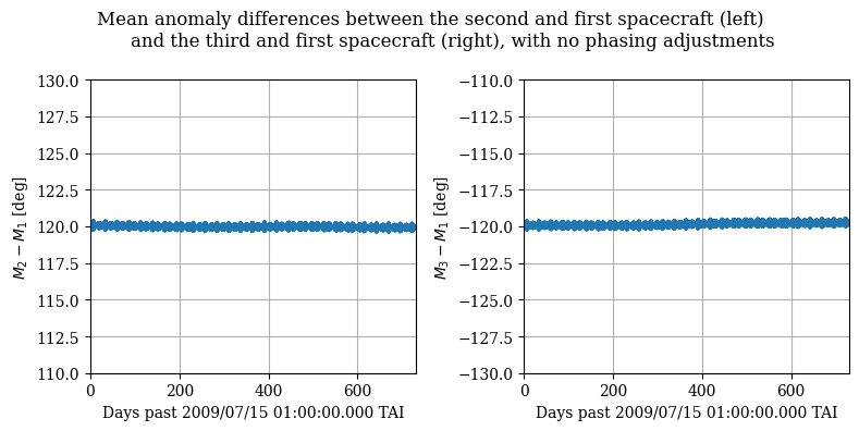
As we can see, the secular drift in the mean anomaly is compensated, and the satellites will maintain the desired separation, and thus coverage, of the South Pole.

South pole coverage statistics

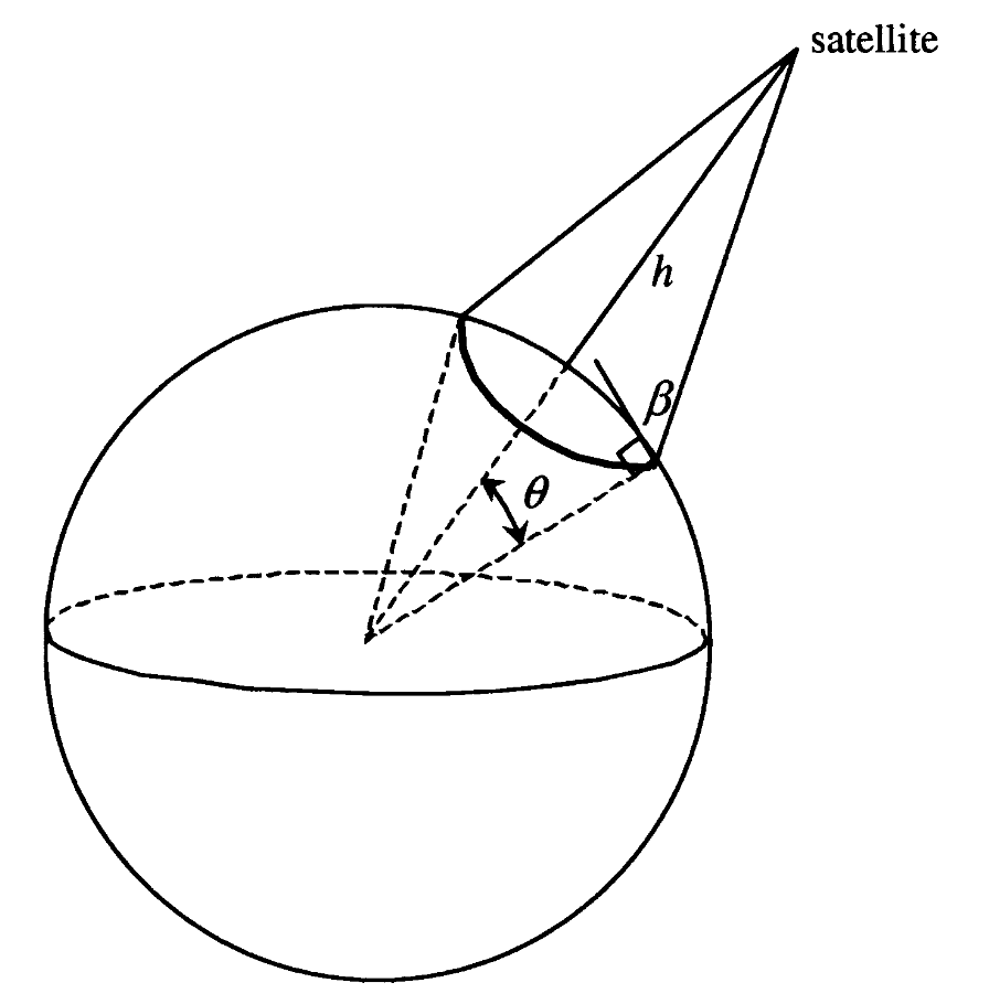
Let’s now compute the coverage statistics of the South Pole by defining a minimum elevation angle of 10 degrees. We will propagate the orbits of the three satellites and whether they are visible.

min_elevation = 10 * pnt.RAD  # [rad] Minimum elevation angle

# Satellite positions in the ME rotating frame
rs_me = np.zeros((n_sat, n_steps_cov, 3))
for i in range(3):
    rs_me[i] = pnt.convert_frame(
        tfs_cov, rvs_mi_adjusted[i], pnt.MOON_CI, pnt.MOON_ME, rotate_only=True
    )[..., :3]

# Visibility
r_south_pole = pnt.lat_lon_alt2cart(np.array([-90 * pnt.RAD, 0, 0]), pnt.R_MOON)
visibility = np.zeros((n_sat, n_steps_cov))
for i in range(3):
    elevation_i = pnt.cart2az_el_range(rs_me[i, :], r_south_pole)[:, 1]
    visibility[i] = elevation_i >= min_elevation

# Metrics
mean_pass = np.zeros(3)
mean_gap = np.zeros(3)
coverage = np.zeros(3)
for i in range(3):
    n_passes = np.sum(np.diff(np.concatenate(([0], visibility[i], [0]))) > 0)
    coverage[i] = np.sum(visibility[i]) / n_steps_cov * 100
    mean_pass[i] = coverage[i] / 100 * dt_total_cov / n_passes / pnt.SECS_HOUR
    mean_gap[i] = (
        (1 - coverage[i] / 100) * dt_total_cov / (n_passes - 1) / pnt.SECS_HOUR
    )

one_fold_coverage = np.sum(np.sum(visibility, axis=0) >= 1) / n_steps_cov * 100
two_fold_coverage = np.sum(np.sum(visibility, axis=0) >= 2) / n_steps_cov * 100

print(f"Mean pass duration: {mean_pass.round(3)} h")
print(f"Mean gap duration:  {mean_gap.round(3)} h")
print(f"Coverage:           {coverage.round(2)} %")
print(f"One-fold coverage:  {one_fold_coverage:.2f} %")
print(f"Two-fold coverage:  {two_fold_coverage:.2f} %")

Mean pass duration: [9.632 9.644 9.636] h
Mean gap duration:  [3.543 3.53  3.529] h
Coverage:           [73.12 73.22 73.21] %
One-fold coverage:  100.00 %
Two-fold coverage:  100.00 %

The computation of the mean pass for the specified satellite is the average of its individual passes over the ten-year propagation period; the mean gap is the average period between passes for the specified satellite; and the percent coverage is the ratio of the sum of the passes over the entire period. Regarding the one- and two-fold constellation statistics, the one-fold mean pass is the average time at least one satellite is in view, and the two-fold mean pass is the average time at least two satellites are in view. Similarly, the mean gap is the average time one or two satellites of the constellation are not in view. The constellation has the desired single and double-fold coverage over the entire span.

Surface Coverage

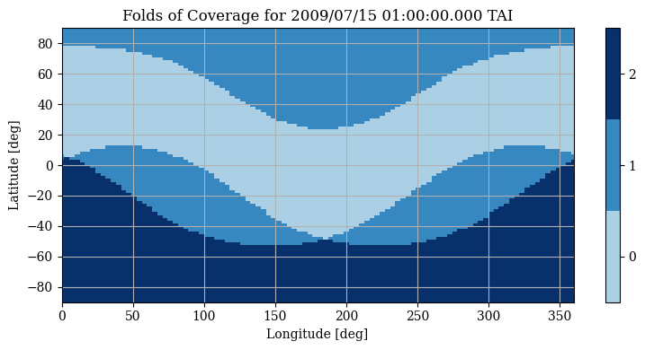
An example of the folds of coverage over the entire planet at the initial epoch is illustrated below, clearly showing the two-fold coverage at the South Pole. The coverage at higher latitudes is very dynamic in time; thus, general conclusions can not be drawn from this single snapshot. Feel free to change the n_steps_fold to see how the one- and two-fold coverage evolves as we consider more steps.

n_steps_fold = 1  # Try 1, 10, 100, 1000

# Surface position
lat = np.linspace(-90, 90, 100) * pnt.RAD
lon = np.linspace(0, 360, 100) * pnt.RAD
lats_mesh, lons_mesh = np.meshgrid(lat, lon)
lats = lats_mesh.flatten()
lons = lons_mesh.flatten()
alts = np.zeros_like(lats)

r_surface = pnt.lat_lon_alt2cart(np.array([lats, lons, alts]).T, pnt.R_MOON)

from tqdm import tqdm

folds_coverage = np.zeros(len(r_surface), dtype=int)
for i, r in tqdm(enumerate(r_surface), total=len(r_surface), desc="Computing coverage"):
    vis_i = np.zeros((n_sat, n_steps_fold), dtype=bool)
    for j in range(3):
        vis_i[j] = (
            pnt.cart2az_el_range(rs_me[j, :n_steps_fold, :3], r)[..., 1]
            >= min_elevation
        )
    folds_coverage[i] = np.min(np.sum(vis_i, axis=0))

folds_coverage = folds_coverage.reshape(len(lat), len(lon))

plt.figure(figsize=(8, 4))
plt.xlim(0, 360)
plt.ylim(-90, 90)
plt.xlabel("Longitude [deg]")
plt.ylabel("Latitude [deg]")
mat = plt.pcolormesh(
    lons_mesh * pnt.DEG,
    lats_mesh * pnt.DEG,
    folds_coverage,
    cmap=cov_cmap,
    vmin=-0.5,
    vmax=n_sat - 0.5,
)
plt.colorbar(mat, ticks=np.arange(n_sat))
plt.title(f"Folds of Coverage for {pnt.time2gregorian_string(t0)} TAI")
plt.grid()
plt.tight_layout()
plt.show()

Computing coverage: 100%|██████████| 10000/10000 [00:00<00:00, 85688.45it/s]

color = pnt.plot.plotly_colors[1]
fig = go.Figure()
pnt.plot.scatter(
    fig, r_surface, color=cov_cmap.colors[folds_coverage.flatten(), :], size=5
)
pnt.plot.plot_orbits(fig, rs_me[:, :n_steps_fold], t=0, marker_size=5, color=color)
pnt.plot.set_view(fig, azimuth=-35, elevation=10, zoom=3)
# Add legend
fig.add_scatter3d(
    x=[0],
    y=[0],
    z=[0],
    mode="markers",
    marker=dict(size=10, color=color),
    name="Satellites",
)
fig.update_layout(width=400, height=400)
fig.show()