Example 15: Mars PNT — a Walker navigation constellation around Mars
LuPNT is designed for lunar Position, Navigation and Timing, but nothing in its core is Moon-specific: the body models, spherical-harmonic gravity, coordinate frames, numerical dynamics, plotting, and time systems all generalize to any central body. This tutorial demonstrates that by building a small Mars navigation constellation end to end — using LuPNT’s native NBodyDynamics propagator and Mars reference frames throughout — and evaluating how well it would let a surface user fix
their position.
We will
build a Mars force model from LuPNT’s higher-order gravity field (
Body.Mars, degree/order \(8\times8\) from the shippedMars50c.cof),use LuPNT’s native Mars frames —
MARS_CI(inertial) andMARS_FIXED(body-fixed) — for propagation and ground tracks,lay out a 9-satellite, 3-plane Walker constellation and propagate it with
NBodyDynamics,visualize the 3-D orbits and the repeating ground tracks with LuPNT’s Plotly routines,
map the median PDOP over the whole surface across several orbits, and
run a user-positioning simulation — pseudorange least squares — at Jezero Crater.
The workflow is identical to the lunar examples; only the central body changes. Every piece of physics — gravity, frame rotation, integration — runs inside LuPNT.
0. Imports and Mars body data
LuPNT’s Body.Mars gives Mars’ gravitational parameter and mean radius, and (as of the planet-frame support) pnt.plot.plot_body and pnt.convert_frame understand Mars directly. We also grab Mars’ shipped surface texture for the 2-D maps later on.
[1]:
import os, sys
from pathlib import Path

import numpy as np
import matplotlib.pyplot as plt
import plotly.graph_objects as go
from PIL import Image

# Use THIS repo's pylupnt/data (mirrors the other tutorials).
for _b in [Path.cwd(), *Path.cwd().parents]:
    if (_b / "python/pylupnt/__init__.py").exists():
        sys.path.insert(0, str((_b / "python").resolve()))
        if (_b / "data/LuPNT_data/ephemeris").is_dir():
            os.environ["LUPNT_DATA_PATH"] = str((_b / "data/LuPNT_data").resolve())
        break
import pylupnt as pnt

np.set_printoptions(precision=4, suppress=True)
RAD, DEG = pnt.RAD, pnt.DEG
LUPNT_DATA = os.environ["LUPNT_DATA_PATH"]

# --- Mars constants from LuPNT's body model ---------------------------------
mars_pm = pnt.Body.Mars()  # point-mass body, for GM / R
GM_MARS = float(mars_pm.GM)  # [m^3/s^2]
R_MARS = float(mars_pm.R)  # [m]  mean volumetric radius (3396 km)

# Mars' sidereal rotation period, from the IAU prime-meridian rate LuPNT uses.
W_DOT_MARS = 350.89198226  # [deg/day]
SIDEREAL_DAY = 360.0 / W_DOT_MARS * pnt.SECS_DAY  # [s]

# Surface texture (shipped with LuPNT) for the 2-D ground-track / DOP maps.
MARS_MAP = np.asarray(Image.open(os.path.join(LUPNT_DATA, "topo", "mars_surface.jpg")))

print(f"GM_MARS       = {GM_MARS:.6e} m^3/s^2")
print(f"R_MARS        = {R_MARS/1e3:.1f} km")
print(f"Sidereal day  = {SIDEREAL_DAY/3600:.4f} h   (Mars: 24.6229 h)")
print(f"Mars frames   : {mars_pm.inertial_frame}  /  {mars_pm.fixed_frame}")

# Host heavy interactive figures on lupnt-doc-assets instead of embedding them.
import sys as _sys
from pathlib import Path as _Path

for _p in [_Path.cwd(), *_Path.cwd().parents]:
    if (_p / "python" / "examples" / "_doc_assets.py").exists():
        _sys.path.insert(0, str(_p / "python" / "examples"))
        break
from _doc_assets import embed_plotly, embed_cesium_scene
[00.01][PyLuPNT] Initializing
GM_MARS       = 4.282838e+13 m^3/s^2
R_MARS        = 3396.0 km
Sidereal day  = 24.6230 h   (Mars: 24.6229 h)
Mars frames   : Frame.MARS_CI  /  Frame.MARS_FIXED
1. Mars’ higher-order gravity field
A navigation constellation lives or dies by how well we know where the satellites are, which is governed by the gravity field. Mars is noticeably less spherical than Earth — its oblateness \(J_2\approx1.96\times10^{-3}\) is about twice Earth’s — so a point-mass model would let the orbits (and the broadcast ephemeris) drift.
Body.Mars(n, m, gravity_file) loads the Mars-50c spherical-harmonic field that LuPNT ships (data/LuPNT_data/gravity/mars/Mars50c.cof, degree/order 50) and keeps it to the degree/order we ask for. We use \(8\times8\), which captures the dominant oblateness and the largest longitude-dependent (tesseral) terms while staying fast. We then build an NBodyDynamics force model around it — the same class the lunar tutorials use, just with a Mars body.
[2]:
N_GRAV = 8  # spherical-harmonic degree/order of the Mars field

mars = pnt.Body.Mars(N_GRAV, N_GRAV, gravity_file="Mars50c.cof")

dyn = pnt.NBodyDynamics()
dyn.set_frame(mars.inertial_frame)  # MARS_CI (Mars-centered inertial, ICRF-aligned)
dyn.set_units(pnt.SI_UNITS)
dyn.add_body(mars)  # Mars 8x8 gravity field
dyn.set_integrator(pnt.IntegratorType.RKF45)
params = pnt.IntegratorParams()
params.reltol = 1e-11
params.abstol = 1e-3  # [m]
dyn.set_integrator_params(params)

# Satellites orbit at ~15,000 km; the Sun's third-body pull and solar radiation pressure there are
# 4-5 orders of magnitude below J2, so the Mars field alone sets the geometry over a few sols.
print(
    "Force model:", [b.name for b in dyn.get_bodies()], f"(gravity {N_GRAV}x{N_GRAV})"
)
Force model: ['MARS'] (gravity 8x8)
How big are the higher-order terms?
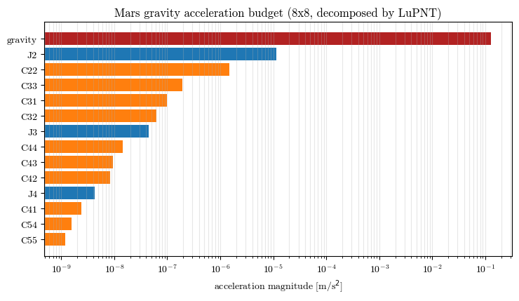
NBodyDynamics.compute_accelerations(..., decompose_gravity=True) splits the total acceleration into the point-mass term plus each individual spherical-harmonic contribution (MARS_J2, MARS_C22, …). Evaluated on a representative satellite, this is the acceleration budget the constellation actually experiences: \(J_2\) sits four orders of magnitude below the central term but acts secularly — it steadily rotates each orbit plane — so it dominates the long-term geometry, while the
tesseral and higher zonal terms add the smaller longitude-dependent structure a repeating ground track feels.
[3]:
# a representative satellite state at the design altitude (in MARS_CI)
r_demo = np.array([R_MARS + 15000e3, 0.0, 0.0, 0.0, 2400.0, 2400.0])
t_demo = pnt.gregorian_to_time(2035, 1, 1, 0, 0, 0)

acc = dyn.compute_accelerations(t_demo, r_demo, decompose_gravity=True)
mags = {name: float(np.linalg.norm(vec)) for name, vec in acc.items()}
ranked = sorted(mags, key=mags.get, reverse=True)

print("Acceleration budget on a satellite at R_Mars + 15,000 km:")
for name in ranked[:8]:
    print(f"  {name:16s} |a| = {mags[name]:.3e} m/s^2")

# horizontal bar chart of the strongest terms (log scale)
show = [n for n in ranked if mags[n] > 0][:14]
labels = [n.replace("MARS_", "") for n in show]
fig, ax = plt.subplots(figsize=(7.5, 4.4))
colors = [
    (
        "#b22222"
        if n == "MARS_gravity"
        else ("#1f77b4" if n.startswith("MARS_J") else "#ff7f0e")
    )
    for n in show
]
ax.barh(range(len(show)), [mags[n] for n in show], color=colors)
ax.set_yticks(range(len(show)))
ax.set_yticklabels(labels)
ax.invert_yaxis()
ax.set_xscale("log")
ax.set_xlabel(r"acceleration magnitude [m/s$^2$]")
ax.set_title("Mars gravity acceleration budget (8x8, decomposed by LuPNT)")
ax.grid(True, axis="x", which="both", alpha=0.3)
plt.tight_layout()
plt.show()
Acceleration budget on a satellite at R_Mars + 15,000 km:
  MARS_gravity     |a| = 1.266e-01 m/s^2
  MARS_J2          |a| = 1.132e-05 m/s^2
  MARS_C22         |a| = 1.485e-06 m/s^2
  MARS_C33         |a| = 1.932e-07 m/s^2
  MARS_C31         |a| = 9.849e-08 m/s^2
  MARS_C32         |a| = 6.208e-08 m/s^2
  MARS_J3          |a| = 4.490e-08 m/s^2
  MARS_C44         |a| = 1.445e-08 m/s^2
2. Mars reference frames
LuPNT defines, for Mars, a Mars-centered inertial frame MARS_CI (ICRF-aligned axes) and a body-fixed frame MARS_FIXED that co-rotates with the surface, using the IAU orientation model. convert_frame moves states and directions between them — exactly as it does for MOON_CI / MOON_PA.
We can read the rotation rate straight out of the frame conversion: sampling the MARS_CI→MARS_FIXED rotation at two epochs and measuring the angle swept about the pole recovers the Martian sidereal day.
[4]:
CI, FIXED = mars.inertial_frame, mars.fixed_frame


def rot_ci_to_fixed(t):
    """MARS_CI -> MARS_FIXED rotation matrix, assembled from LuPNT's convert_frame."""
    cols = [np.asarray(pnt.convert_frame(t, e, CI, FIXED, True)) for e in np.eye(3)]
    return np.column_stack(cols)


t0 = pnt.gregorian_to_time(2035, 1, 1, 0, 0, 0)
R0 = rot_ci_to_fixed(t0)
R1 = rot_ci_to_fixed(t0 + 3600.0)
dR = R1 @ R0.T  # incremental spin over 1 h
angle = np.arccos(np.clip((np.trace(dR) - 1.0) / 2.0, -1, 1))
period = 2 * np.pi / (angle / 3600.0)
print(f"R orthonormal err : {np.abs(R0 @ R0.T - np.eye(3)).max():.2e}")
print(f"measured Mars day : {period/3600:.4f} h   (sidereal, 24.6229 h)")
R orthonormal err : 2.22e-16
measured Mars day : 24.6230 h   (sidereal, 24.6229 h)
A Mars-equatorial frame for constellation design
MARS_CI is ICRF-aligned (its \(z\)-axis is the ICRF pole, not Mars’ pole — the same convention as MOON_CI). Mars’ spin pole is tilted about \(37^\circ\) from the ICRF pole, so if we built orbital elements directly in MARS_CI, an “inclination” would be measured against the wrong equator.
To design the constellation against Mars’ equator, we build a Mars-equatorial inertial frame from LuPNT’s own Mars orientation: the body-fixed \(z\)-axis is Mars’ pole, so rotating it into MARS_CI gives the pole direction, from which we complete an orthonormal triad. The resulting rotation R_eq2ci maps a state designed in Mars-equatorial coordinates into MARS_CI for propagation.
[5]:
def mars_equatorial_to_ci(t):
    """Rotation from a Mars-equatorial inertial frame (z = Mars pole) to MARS_CI."""
    pole = np.asarray(pnt.convert_frame(t, np.array([0.0, 0.0, 1.0]), FIXED, CI, True))
    pole /= np.linalg.norm(pole)
    x = np.cross([0.0, 0.0, 1.0], pole)  # node of Mars equator on the ICRF equator
    x /= np.linalg.norm(x)
    y = np.cross(pole, x)
    return np.column_stack([x, y, pole])  # columns = equatorial axes in MARS_CI


R_EQ2CI = mars_equatorial_to_ci(t0)
tilt = np.degrees(np.arccos(R_EQ2CI[2, 2]))
print(f"Mars pole tilt from ICRF pole: {tilt:.2f} deg")
Mars pole tilt from ICRF pole: 37.13 deg
3. A 9-satellite Walker constellation
We use a Walker :math:`delta` pattern \(T/P/F\): \(T=9\) satellites in \(P=3\) planes (RAAN steps of \(120^\circ\)), \(F=1\) setting the inter-plane phase, all sharing a circular orbit at \(45^\circ\) inclination (w.r.t. Mars’ equator). We size the orbit at 15,000 km altitude — high enough that each satellite sees a wide cap of the surface (nine satellites is a minimal fleet), with a \(\sim21\) h period that is deliberately not synchronous with the 24.6 h Martian day, so the ground tracks slowly walk westward and every longitude is sampled over a few sols.
Each satellite’s classical elements are turned into a Cartesian state with LuPNT’s classical_to_cart (in the Mars-equatorial frame) and then rotated into MARS_CI for propagation.
[6]:
N_SAT, N_PLANES, F_WALKER = 9, 3, 1
SATS_PER_PLANE = N_SAT // N_PLANES
ALT = 15000e3
A_SMA = R_MARS + ALT
INC = 45.0 * RAD
PERIOD = 2 * np.pi * np.sqrt(A_SMA**3 / GM_MARS)
EPOCH = t0


def walker_elements(T, P, Fp, a, e, inc):
    """Classical elements [a,e,i,RAAN,argp,M] for a Walker-delta constellation."""
    spp = T // P
    coes = []
    for p in range(P):
        raan = p * 2 * np.pi / P
        for s in range(spp):
            M = (s * 2 * np.pi / spp + p * 2 * np.pi * Fp / T) % (2 * np.pi)
            coes.append([a, e, inc, raan, 0.0, M])
    return np.array(coes)


COES = walker_elements(N_SAT, N_PLANES, F_WALKER, A_SMA, 0.0, INC)

# element -> Cartesian (Mars-equatorial) -> MARS_CI
RV0 = np.zeros((N_SAT, 6))
for k, coe in enumerate(COES):
    rv_eq = pnt.classical_to_cart(coe, GM_MARS)
    RV0[k, :3] = R_EQ2CI @ rv_eq[:3]
    RV0[k, 3:] = R_EQ2CI @ rv_eq[3:]

print(f"Walker {N_SAT}/{N_PLANES}/{F_WALKER} constellation")
print(
    f"  {N_PLANES} planes x {SATS_PER_PLANE} sats,  inclination {INC*DEG:.0f} deg (Mars equator)"
)
print(f"  altitude {ALT/1e3:.0f} km  (a = {A_SMA/1e3:.0f} km)")
print(f"  orbital period {PERIOD/3600:.2f} h  vs Martian day {SIDEREAL_DAY/3600:.2f} h")
Walker 9/3/1 constellation
  3 planes x 3 sats,  inclination 45 deg (Mars equator)
  altitude 15000 km  (a = 18396 km)
  orbital period 21.04 h  vs Martian day 24.62 h
Propagate over several orbits with NBodyDynamics
We propagate all nine satellites for two Martian sols (a little over two orbital periods) at 3-minute sampling, entirely with LuPNT’s NBodyDynamics.propagate under the \(8\times8\) Mars field. Rotating the inertial states into MARS_FIXED with convert_frame gives the body-fixed positions used for ground tracks and user geometry.
[7]:
T_SIM = 2 * SIDEREAL_DAY
DT = 180.0
TS = EPOCH + np.arange(0.0, T_SIM, DT)
N_T = len(TS)

POS_CI = np.zeros((N_SAT, N_T, 3))
for k in range(N_SAT):
    POS_CI[k] = np.asarray(dyn.propagate(RV0[k], TS))[:, :3]

# inertial -> body-fixed (pure rotation about the shared Mars center)
POS_FIXED = np.zeros((N_SAT, N_T, 3))
for k in range(N_SAT):
    POS_FIXED[k] = np.asarray(pnt.convert_frame(TS, POS_CI[k], CI, FIXED, True))

r_norm = np.linalg.norm(POS_CI, axis=2)
print(
    f"Propagated {N_SAT} satellites over {T_SIM/SIDEREAL_DAY:.1f} sols "
    f"({N_T} epochs, {T_SIM/PERIOD:.1f} orbital periods)"
)
print(
    f"orbit-radius spread [km]: {(r_norm.max()-r_norm.min())/1e3:.1f}  (short-period J2 breathing)"
)
Propagated 9 satellites over 2.0 sols (985 epochs, 2.3 orbital periods)
orbit-radius spread [km]: 6.9  (short-period J2 breathing)
4. The constellation in 3-D
LuPNT’s Plotly helpers render the scene: plot_body draws the textured Mars globe (Mars is a first-class body in the plot module now) and plot_orbits draws the trajectories — the same routines the lunar tutorials use.
[8]:
n_one = int(np.ceil(PERIOD / DT))  # ~one orbital period, so the plot is not overcrowded
colors = ["#e6194B", "#3cb44b", "#4363d8"]  # one colour per plane

fig = go.Figure()
pnt.plot.plot_body(fig, pnt.MARS, size_factor=6)
for k in range(N_SAT):
    pnt.plot.plot_orbits(fig, POS_CI[k, :n_one], color=colors[k // SATS_PER_PLANE])
fig.add_scatter3d(
    x=POS_CI[:, 0, 0] / 1e6,
    y=POS_CI[:, 0, 1] / 1e6,
    z=POS_CI[:, 0, 2] / 1e6,
    mode="markers",
    marker=dict(size=4, color="black"),
    name="satellites",
)
pnt.plot.set_view(fig, azimuth=40, elevation=22, zoom=2.6)
fig.update_layout(
    width=620,
    height=620,
    title=f"Mars Walker {N_SAT}/{N_PLANES}/{F_WALKER} constellation (MARS_CI, one period)",
)
embed_plotly(fig, "ex15_marspnt")
[doc-asset] plots/ex15_marspnt.html (5648 kB) -> https://stanford-navlab.github.io/lupnt-doc-assets/plots/ex15_marspnt.html
5. Ground tracks
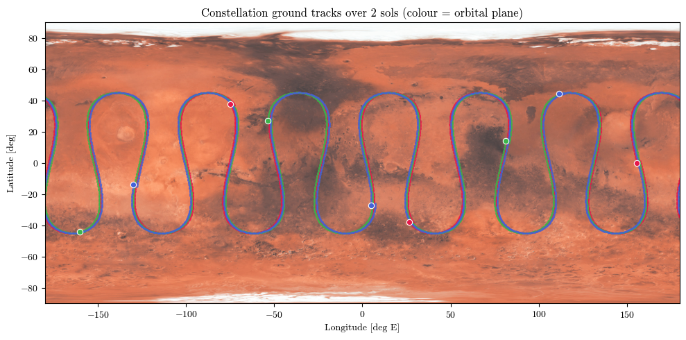
Reading planetocentric latitude/longitude off the body-fixed positions (LuPNT’s cart_to_lat_lon_alt, which returns degrees) gives the ground tracks. Because the orbital period is close to — but not equal to — the Martian day, each track is a slowly drifting sinusoid reaching \(\pm45^\circ\) latitude, the three planes offset by \(120^\circ\) in longitude.
[9]:
lla = np.array(
    [np.asarray(pnt.cart_to_lat_lon_alt(POS_FIXED[k], R_MARS)) for k in range(N_SAT)]
)

fig, ax = plt.subplots(figsize=(10, 5))
ax.imshow(
    MARS_MAP, extent=[-180, 180, -90, 90], aspect="auto", origin="upper", alpha=0.85
)
for k in range(N_SAT):
    lon = ((lla[k, :, 1] + 180.0) % 360.0) - 180.0
    ax.scatter(lon, lla[k, :, 0], s=1.5, color=colors[k // SATS_PER_PLANE], alpha=0.5)
for k in range(N_SAT):
    lon0 = ((lla[k, 0, 1] + 180.0) % 360.0) - 180.0
    ax.plot(
        lon0,
        lla[k, 0, 0],
        "o",
        ms=6,
        color=colors[k // SATS_PER_PLANE],
        mec="white",
        mew=0.8,
    )
ax.set_xlim(-180, 180)
ax.set_ylim(-90, 90)
ax.set_xlabel("Longitude [deg E]")
ax.set_ylabel("Latitude [deg]")
ax.set_title("Constellation ground tracks over 2 sols (colour = orbital plane)")
plt.tight_layout()
plt.show()
6. Coverage and DOP across the surface
For a surface user, positioning accuracy is range-measurement noise multiplied by the dilution of precision. With line-of-sight unit vectors \(\hat{\mathbf u}_i\) (in the user’s local East-North-Up frame) to the visible satellites, the geometry matrix stacks rows \([\hat u_E,\hat u_N,\hat u_U,1]\) (the last column solving for the receiver clock), and
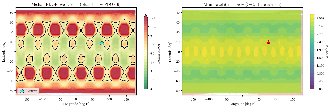
A fix needs at least four satellites above the elevation mask. We sweep a \(5^\circ\times5^\circ\) grid, compute PDOP at every epoch, and map the median PDOP over the two-sol window — the typical geometry a user at each location would experience.
[10]:
MASK_DEG = 5.0
MASK = np.deg2rad(MASK_DEG)


def pdop_stack(u_enu, visible):
    """Vectorized PDOP over (..., n_sat, 3) LOS unit vectors + boolean visibility."""
    H = np.concatenate([u_enu, np.ones(u_enu.shape[:-1] + (1,))], axis=-1)
    Hw = H * visible[..., None]
    M = np.einsum("...sa,...sb->...ab", Hw, H)
    bad = visible.sum(axis=-1) < 4
    M[bad] = np.eye(4)
    Minv = np.linalg.inv(M)
    pdop = np.sqrt(
        np.clip(Minv[..., 0, 0] + Minv[..., 1, 1] + Minv[..., 2, 2], 0.0, None)
    )
    pdop[bad] = np.nan
    return pdop


LAT_G = np.arange(-85.0, 85.1, 5.0)
LON_G = np.arange(-180.0, 180.0, 5.0)
med_pdop = np.full((len(LAT_G), len(LON_G)), np.nan)
mean_vis = np.zeros_like(med_pdop)

for i, la in enumerate(LAT_G):  # loop latitudes (keeps memory small)
    lo = np.deg2rad(LON_G)
    lar = np.deg2rad(la)
    E = np.stack([-np.sin(lo), np.cos(lo), np.zeros_like(lo)], -1)
    Nn = np.stack(
        [
            -np.sin(lar) * np.cos(lo),
            -np.sin(lar) * np.sin(lo),
            np.full_like(lo, np.cos(lar)),
        ],
        -1,
    )
    Up = np.stack(
        [
            np.cos(lar) * np.cos(lo),
            np.cos(lar) * np.sin(lo),
            np.full_like(lo, np.sin(lar)),
        ],
        -1,
    )
    ru = R_MARS * Up
    los = POS_FIXED[None, :, :, :] - ru[:, None, None, :]  # (nlon,nsat,nT,3)
    e = np.einsum("lc,lstc->lst", E, los)
    n = np.einsum("lc,lstc->lst", Nn, los)
    u = np.einsum("lc,lstc->lst", Up, los)
    rng = np.sqrt(e**2 + n**2 + u**2)
    vis = np.arcsin(np.clip(u / rng, -1, 1)) >= MASK
    u_enu = np.moveaxis(
        np.stack([e / rng, n / rng, u / rng], -1), 1, 2
    )  # (nlon,nT,nsat,3)
    vis_t = np.moveaxis(vis, 1, 2)
    med_pdop[i] = np.nanmedian(pdop_stack(u_enu, vis_t), axis=1)
    mean_vis[i] = vis.sum(1).mean(1)

print(f"Global median PDOP  : {np.nanmedian(med_pdop):.2f}")
print(
    f"Grid fraction with median PDOP < 6 : {np.mean(med_pdop[~np.isnan(med_pdop)] < 6)*100:.0f}%"
)
print(f"Mean satellites in view (grid avg) : {mean_vis.mean():.2f}")
Global median PDOP  : 6.74
Grid fraction with median PDOP < 6 : 37%
Mean satellites in view (grid avg) : 3.27
[11]:
JEZERO = (18.44, 77.45)  # Perseverance rover site (lat N, lon E)

fig, axes = plt.subplots(1, 2, figsize=(14, 4.6))

ax = axes[0]
ax.imshow(
    MARS_MAP, extent=[-180, 180, -90, 90], aspect="auto", origin="upper", alpha=0.35
)
pdop_clip = np.clip(med_pdop, 0, 12)
cf = ax.contourf(
    LON_G,
    LAT_G,
    pdop_clip,
    levels=np.linspace(0, 12, 25),
    cmap="RdYlGn_r",
    alpha=0.75,
    extend="max",
)
ax.contour(LON_G, LAT_G, pdop_clip, levels=[6], colors="k", linewidths=1.2)
ax.plot(
    JEZERO[1], JEZERO[0], "*", ms=16, color="cyan", mec="k", mew=0.6, label="Jezero"
)
ax.set_title("Median PDOP over 2 sols  (black line = PDOP 6)")
ax.set_xlabel("Longitude [deg E]")
ax.set_ylabel("Latitude [deg]")
ax.legend(loc="lower left")
plt.colorbar(cf, ax=ax, label="median PDOP", shrink=0.85)

ax = axes[1]
ax.imshow(
    MARS_MAP, extent=[-180, 180, -90, 90], aspect="auto", origin="upper", alpha=0.35
)
cf2 = ax.contourf(
    LON_G,
    LAT_G,
    mean_vis,
    levels=np.linspace(0, mean_vis.max(), 20),
    cmap="viridis",
    alpha=0.8,
)
ax.plot(JEZERO[1], JEZERO[0], "*", ms=16, color="red", mec="k", mew=0.6)
ax.set_title("Mean satellites in view (>= 5 deg elevation)")
ax.set_xlabel("Longitude [deg E]")
ax.set_ylabel("Latitude [deg]")
plt.colorbar(cf2, ax=ax, label="# visible", shrink=0.85)

plt.tight_layout()
plt.show()
7. User positioning at Jezero Crater
Finally we simulate what a surface user actually gets. At Jezero Crater (Perseverance’s landing site, \(18.44^\circ\)N, \(77.45^\circ\)E) we form a pseudorange to every visible satellite,
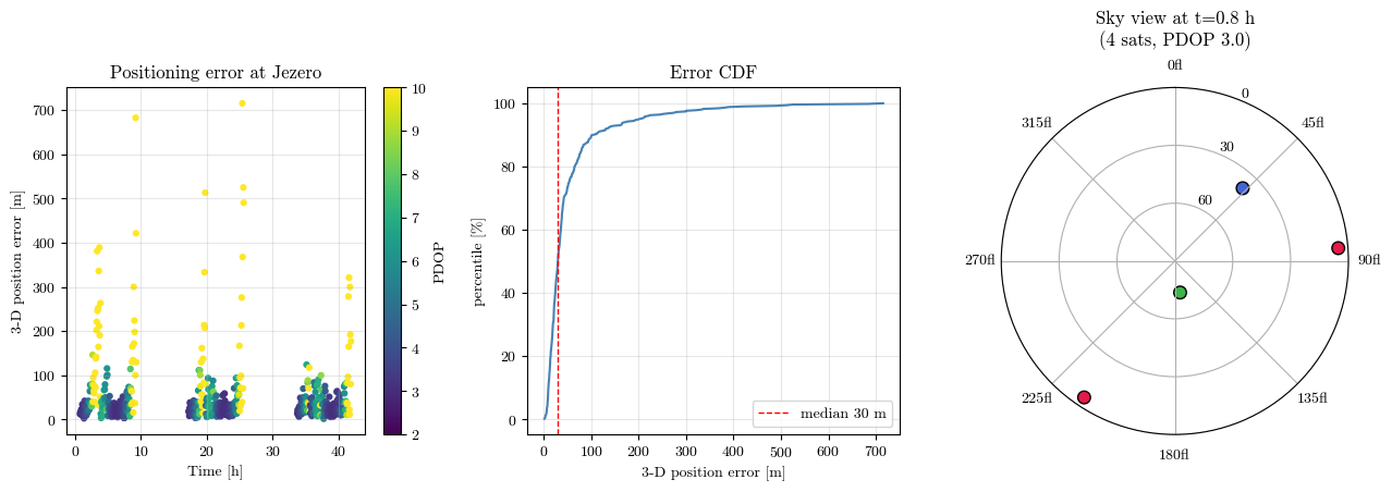
with a single unknown clock bias \(c\,\delta t\) and \(\sigma=8\) m ranging noise. At each epoch with four or more satellites in view we solve for position and clock by iterated (Gauss–Newton) least squares, starting from the planet center, and compare against the known truth.
[12]:
def enu_basis(lat, lon):
    cl, sl, co, so = np.cos(lat), np.sin(lat), np.cos(lon), np.sin(lon)
    return np.array([[-so, co, 0.0], [-sl * co, -sl * so, cl], [cl * co, cl * so, sl]])


lat_u, lon_u = np.deg2rad(JEZERO[0]), np.deg2rad(JEZERO[1])
r_user = R_MARS * np.array(
    [np.cos(lat_u) * np.cos(lon_u), np.cos(lat_u) * np.sin(lon_u), np.sin(lat_u)]
)
Renu = enu_basis(lat_u, lon_u)

los = POS_FIXED - r_user[None, None, :]
enu = np.einsum("ij,ktj->kti", Renu, los)
rng_u = np.linalg.norm(enu, axis=-1)
elev_u = np.arcsin(np.clip(enu[..., 2] / rng_u, -1, 1))
az_u = np.arctan2(enu[..., 0], enu[..., 1])
vis_u = elev_u >= MASK

SIGMA = 8.0
rng_gen = np.random.default_rng(42)

err3d, err_h, err_v, epochs_fix, pdop_fix = [], [], [], [], []
for tt in range(N_T):
    m = vis_u[:, tt]
    if m.sum() < 4:
        continue
    sats = POS_FIXED[m, tt, :]
    rho = (
        np.linalg.norm(sats - r_user, axis=1) + rng_gen.standard_normal(m.sum()) * SIGMA
    )
    x = np.zeros(4)  # [x, y, z, c*dt]
    for _ in range(15):
        d = x[:3] - sats
        r = np.linalg.norm(d, axis=1)
        H = np.concatenate([d / r[:, None], np.ones((m.sum(), 1))], axis=1)
        dx = np.linalg.lstsq(H, rho - (r + x[3]), rcond=None)[0]
        x += dx
        if np.linalg.norm(dx[:3]) < 1e-3:
            break
    derr = Renu @ (x[:3] - r_user)
    err3d.append(np.linalg.norm(derr))
    err_h.append(np.hypot(derr[0], derr[1]))
    err_v.append(abs(derr[2]))
    epochs_fix.append((TS[tt] - EPOCH) / 3600.0)
    Q = np.linalg.inv(H.T @ H)
    pdop_fix.append(np.sqrt(Q[0, 0] + Q[1, 1] + Q[2, 2]))

err3d = np.array(err3d)
err_h = np.array(err_h)
err_v = np.array(err_v)
pdop_fix = np.array(pdop_fix)
epochs_fix = np.array(epochs_fix)

print(
    f"Epochs with >= 4 satellites : {len(err3d)} / {N_T} ({100*len(err3d)/N_T:.0f}% of the window)"
)
print(
    f"3-D position error   median {np.median(err3d):6.1f} m   95% {np.percentile(err3d,95):6.1f} m"
)
print(f"  horizontal         median {np.median(err_h):6.1f} m")
print(f"  vertical           median {np.median(err_v):6.1f} m")
print(f"PDOP at fix epochs    median {np.median(pdop_fix):.2f}")
Epochs with >= 4 satellites : 504 / 985 (51% of the window)
3-D position error   median   30.0 m   95%  201.6 m
  horizontal         median   15.2 m
  vertical           median   20.0 m
PDOP at fix epochs    median 4.84
[13]:
fig = plt.figure(figsize=(13, 4.4))

ax = fig.add_subplot(1, 3, 1)
sc = ax.scatter(epochs_fix, err3d, c=pdop_fix, cmap="viridis", s=12, vmin=2, vmax=10)
ax.set_xlabel("Time [h]")
ax.set_ylabel("3-D position error [m]")
ax.set_title("Positioning error at Jezero")
ax.grid(alpha=0.3)
plt.colorbar(sc, ax=ax, label="PDOP")

ax = fig.add_subplot(1, 3, 2)
xs = np.sort(err3d)
ys = np.arange(1, len(xs) + 1) / len(xs)
ax.plot(xs, ys * 100, color="steelblue")
ax.axvline(
    np.median(err3d),
    color="red",
    ls="--",
    lw=1,
    label=f"median {np.median(err3d):.0f} m",
)
ax.set_xlabel("3-D position error [m]")
ax.set_ylabel("percentile [%]")
ax.set_title("Error CDF")
ax.grid(alpha=0.3)
ax.legend()

ax = fig.add_subplot(1, 3, 3, projection="polar")
best = np.argmin(pdop_fix)
tt = np.where(np.isclose((TS - EPOCH) / 3600.0, epochs_fix[best]))[0][0]
m = vis_u[:, tt]
ax.set_theta_zero_location("N")
ax.set_theta_direction(-1)
ax.scatter(
    az_u[m, tt],
    90 - np.rad2deg(elev_u[m, tt]),
    c=[colors[k // SATS_PER_PLANE] for k in np.where(m)[0]],
    s=70,
    edgecolors="k",
)
ax.set_rmax(90)
ax.set_rticks([30, 60, 90])
ax.set_yticklabels(["60", "30", "0"])
ax.set_title(
    f"Sky view at t={epochs_fix[best]:.1f} h\n({m.sum()} sats, PDOP {pdop_fix[best]:.1f})",
    va="bottom",
)

plt.tight_layout()
plt.show()
Summary
Using LuPNT’s native machinery end to end, we built a simple Mars-PNT study:
an \(8\times8\) Mars-50c gravity force model via
Body.Mars+NBodyDynamics, whose \(J_2\approx2\times10^{-3}\) drives the constellation geometry (the higher-order terms shown directly bycompute_accelerations);Mars’ native inertial and body-fixed frames (
MARS_CI/MARS_FIXED) viaconvert_frame, with a Mars-equatorial design frame derived from LuPNT’s own Mars pole;a 9/3/1 Walker constellation at 15,000 km, propagated for two sols with
NBodyDynamicsand visualized with LuPNT’s Plotly body/orbit routines;a median-PDOP surface map showing where nine satellites already give a usable fix and where the minimal fleet leaves gaps; and
a pseudorange least-squares positioning simulation at Jezero Crater, reaching tens-of-metres accuracy whenever four or more satellites clear the horizon.