Example 2: Relativistic Time Conversions – TT, TCL, and LT
This tutorial shows how LuPNT handles relativistic time scales for cislunar navigation. The goal is both practical and mathematical: use LuPNT time-conversion routines, then reproduce the main secular and periodic terms with a vectorized Python implementation.
The key idea is that a clock rate depends on the gravitational potential and velocity of the reference frame. Earth-centered, barycentric, selenocentric, and lunar-surface time scales therefore do not remain exactly synchronized.
Scale |
Reference environment |
Interpretation |
|---|---|---|
TT |
Earth geoid |
Terrestrial time; related to TAI by TT = TAI + 32.184 s |
TCG |
Geocentric coordinate frame |
Coordinate time for the GCRS |
TCB |
Solar-system barycentric frame |
Coordinate time for the BCRS |
TDB |
Barycentric, scaled |
Scaled form of TCB that stays close to TT on average |
TCL |
Selenocentric coordinate frame |
Coordinate time centered on the Moon |
LT |
Lunar surface |
Lunar analogue of TT, tied to the lunar geoid |
All scales are aligned at the conventional reference epoch \(T_0=\text{1977-01-01 00:00:32.184 TAI}\).
The constants used below are:
\(L_G = 6.969290134 \times 10^{-10}\) for TCG-TT,
\(L_B = 1.550519768 \times 10^{-8}\) for TCB-TDB,
\(L_L = 3.13905 \times 10^{-11}\) for TCL-LT,
\(L_{EM} = 1.7093906 \times 10^{-11}\) for the mean LT-TT rate correction.
[1]:
import time
import numpy as np
import matplotlib.pyplot as plt
import matplotlib.ticker as ticker

import os, sys
from pathlib import Path

# Use THIS repo's pylupnt/data, not a stale copy on a global PYTHONPATH (~/.zshrc) or kernelspec.
for _b in [Path.cwd(), *Path.cwd().parents]:
    if (_b / "python/pylupnt/__init__.py").exists():
        sys.path.insert(0, str((_b / "python").resolve()))
        if (_b / "data/LuPNT_data/ephemeris").is_dir():
            os.environ["LUPNT_DATA_PATH"] = str((_b / "data/LuPNT_data").resolve())
        break
import pylupnt as pnt

# --- Fundamental constants ---
L_G = pnt.L_G  # TT-TCG scale: d(TCG-TT)/dTT = L_G/(1-L_G)
L_B = pnt.L_B  # TDB-TCB scale
L_L = pnt.L_L  # LT-TCL scale: LT runs slower than TCL on the lunar geoid
L_EM = 1.7093906e-11  # mean LT-TT rate correction (Fienga+2023; not yet in Python API)
C = 299792458  # speed of light [m/s]
SECS_DAY = pnt.SECS_DAY
TDB_0 = -65.5e-6  # [s] TDB offset (DE405 ephemeris, from LuPNT constants.h)

# Reference epoch T_0 = 1977-01-01 00:00:32.184 TAI
T0_MJD = pnt.MJD_COORDINATE_TT_TCG_TCB  # 43144.0003725
T0_TT = pnt.mjd_to_time(T0_MJD)  # [s] from J2000 in TT
MJD_J2000 = pnt.MJD_J2000_TT  # 51544.5

print(f"Reference epoch T_0: MJD {T0_MJD}  =  {T0_TT:.3f} s from J2000 (TT)")
print(f"L_G={L_G:.4e}, L_B={L_B:.4e}, L_L={L_L:.4e}, L_EM={L_EM:.4e}")
print(f"Speed of light: c = {C:.0f} m/s")
[00.01][PyLuPNT] Initializing
Reference epoch T_0: MJD 43144.0003725  =  -725803167.816 s from J2000 (TT)
L_G=6.9693e-10, L_B=1.5505e-08, L_L=3.1390e-11, L_EM=1.7094e-11
Speed of light: c = 299792458 m/s
1. Analytical secular drift rates
Some time-scale differences are exactly linear by definition. For example,
The mean LT-TT drift combines the geocentric, barycentric, and lunar-surface scalings:
This first section computes those rates directly so the later numerical curves have an expected slope.
[2]:
# TCG-TT: exact linear relationship (IAU Resol. B1.5)
rate_tcg_tt = L_G / (1 - L_G) * SECS_DAY * 1e6  # [us/day]

# LT-TCL: exact linear relationship (Guinot 2011)
rate_lt_tcl = -L_L * SECS_DAY * 1e6  # [us/day]

# LT-TT: analytical secular rate (IERS TN 36)
rate_lt_tt = ((L_G - L_L) / (1 - L_B) - L_EM) * SECS_DAY * 1e6  # [us/day]

print("Analytical secular drift rates")
print("-" * 45)
print(f"  TCG - TT  : {rate_tcg_tt:+.4f}  us/day")
print(f"  LT  - TCL : {rate_lt_tcl:+.4f}  us/day")
print(f"  LT  - TT  : {rate_lt_tt:+.4f}  us/day")
print()
print("Note: TCL-TT secular rate is computed numerically in Section 4.2.")
Analytical secular drift rates
---------------------------------------------
  TCG - TT  : +60.2147  us/day
  LT  - TCL : -2.7121  us/day
  LT  - TT  : +56.0256  us/day

Note: TCL-TT secular rate is computed numerically in Section 4.2.
2. TCL-TT by numerical integration
The selenocentric coordinate time TCL differs from barycentric time because the Moon moves through the solar-system gravitational potential. The defining integral is
LuPNT evaluates this with ephemerides for the Moon, Sun, and planets. The notebook repeats the same computation in vectorized Python: sample the integrand on a dense time grid, integrate with cumulative quadrature, and combine with the TDB-TCB scaling. This exposes the mathematical structure while keeping the calculation fast enough for plotting.
[3]:
# Time grid: T_0 to T_0 + 45 years, step = 0.1 days
dt_day = 0.1
n_years = 45
n_grid = int(n_years * 365.25 / dt_day) + 1
dt = dt_day * SECS_DAY

t_tt_grid = T0_TT + np.arange(n_grid, dtype=np.float64) * dt
days = np.arange(n_grid, dtype=np.float64) * dt_day  # elapsed days from T_0

print(f"Grid: {n_grid:,} points over {n_years} years ({n_grid * dt_day:.1f} days)")
print(f"Step: {dt_day} day = {dt:.0f} s")
Grid: 164,363 points over 45 years (16436.3 days)
Step: 0.1 day = 8640 s
[4]:
# Step 1: TT -> TDB  (Fairhead-Bretagnon expansion, vectorised)
t0_perf = time.time()
t_tdb_grid = pnt.convert_time(t_tt_grid, pnt.Time.TT, pnt.Time.TDB)
print(f"TT->TDB ({n_grid:,} pts): {time.time()-t0_perf:.2f} s")

# Step 2: TDB -> TCB  (matches C++ TtToTcb in time_conversions.cc)
t_tcb_grid = (t_tdb_grid - L_B * T0_TT - TDB_0) / (1.0 - L_B)
dt_tcb = np.diff(t_tcb_grid)  # step sizes for trapezoidal integration
TT->TDB (164,363 pts): 0.00 s
[5]:
# Step 3: Moon state in BCRS (vectorised SPICE, centre = SSB)
t0_perf = time.time()
rv_moon = pnt.get_body_pos_vel(
    t_tdb_grid, pnt.BodyId.SSB, pnt.BodyId.MOON, pnt.Frame.GCRF, pnt.SI_UNITS
)
x_moon = rv_moon[:, :3]  # [m]
v_moon = rv_moon[:, 3:]  # [m/s]
print(f"Moon state ({n_grid:,} pts): {time.time()-t0_perf:.2f} s")

# Step 4: External body potentials (matches C++ kTclExternalBodies in time_conversions.cc)
# GM values match C++ constants.h: planet-only (not barycenter system) values
# Note: for Jupiter/Saturn/Uranus/Neptune the C++ constants are GM_PLANET (planet only),
# which differ from GM_*_SYSTEM (planet + moons) by a small factor for the inner planets
# and a factor used in LuPNT's implementation for the outer planets.
GM_JUPITER_cpp = 0.1267127646799999e17  # C++ GM_JUPITER  [m^3/s^2]
GM_SATURN_cpp = 0.3794058480000000e16  # C++ GM_SATURN   [m^3/s^2]
GM_URANUS_cpp = 0.5794556400000000e15  # C++ GM_URANUS   [m^3/s^2]
GM_NEPTUNE_cpp = 0.6836527100580000e15  # C++ GM_NEPTUNE  [m^3/s^2]
GM_MARS_cpp = 0.4282837566395650e14  # C++ GM_MARS     [m^3/s^2]

kTclExternal = [
    (pnt.BodyId.SUN, pnt.GM_SUN),
    (pnt.BodyId.MERCURY, pnt.GM_MERCURY),
    (pnt.BodyId.VENUS, pnt.GM_VENUS),
    (pnt.BodyId.EARTH, pnt.GM_EARTH),
    (pnt.BodyId.MARS, GM_MARS_cpp),
    (pnt.BodyId.JUPITER, GM_JUPITER_cpp),
    (pnt.BodyId.SATURN_BARYCENTER, GM_SATURN_cpp),
    (pnt.BodyId.URANUS_BARYCENTER, GM_URANUS_cpp),
    (pnt.BodyId.NEPTUNE_BARYCENTER, GM_NEPTUNE_cpp),
]

t0_perf = time.time()
w_ext = np.zeros(n_grid)  # sum GM_A / r_{Moon,A}  [m^2/s^2]
for body_id, gm in kTclExternal:
    rv_b = pnt.get_body_pos_vel(
        t_tdb_grid, pnt.BodyId.SSB, body_id, pnt.Frame.GCRF, pnt.SI_UNITS
    )
    r = np.linalg.norm(x_moon - rv_b[:, :3], axis=1)
    w_ext += gm / r
print(f"External potentials (9 bodies): {time.time()-t0_perf:.2f} s")
Moon state (164,363 pts): 0.28 s
External potentials (9 bodies): 0.26 s
[6]:
# Step 5: TCB->TCL integrand  (matches C++ TcbToTclIntegrandC2)
v2 = np.sum(v_moon**2, axis=1)  # |v_Moon_BCRS|^2  [m^2/s^2]
integrand = 0.5 * v2 + w_ext  # [m^2/s^2]

# Step 6: Trapezoidal forward integration from T_0
integral_c2 = np.zeros(n_grid)
integral_c2[1:] = np.cumsum(0.5 * (integrand[:-1] + integrand[1:]) * dt_tcb)

# Step 7: TCL = TCB - integral/c^2
t_tcl_grid = t_tcb_grid - integral_c2 / C**2
diff_tcl_tt_us = (t_tcl_grid - t_tt_grid) * 1e6  # [us]

# Secular rate from linear fit over 45 years
poly_tcl = np.polyfit(days, diff_tcl_tt_us, 1)
trend_tcl = np.polyval(poly_tcl, days)
periodic_tcl_us = diff_tcl_tt_us - trend_tcl

print("TCL-TT integration results")
print("-" * 50)
print(f"  Secular rate (numerical):    {poly_tcl[0]:+.4f}  us/day")
print(f"  TCL-TT at T_0 (offset):     {diff_tcl_tt_us[0]:+.4f}  us")
print(
    f"  Periodic amplitude (45 yr):  {(periodic_tcl_us.max()-periodic_tcl_us.min())/2:.2f}  us (half p-p)"
)
print(f"  Mean integrand:              {integrand.mean():.6e}  m^2/s^2")
TCL-TT integration results
--------------------------------------------------
  Secular rate (numerical):    +58.9061  us/day
  TCL-TT at T_0 (offset):     +6.4373  us
  Periodic amplitude (45 yr):  162.50  us (half p-p)
  Mean integrand:              1.332270e+09  m^2/s^2
3. Validate against LuPNT ConvertTime
pnt.convert_time / ConvertTime is the production API. The custom vectorized implementation above should agree at representative checkpoints. This comparison is a useful pattern for tutorials: implement the math once in transparent Python, then verify that the library call gives the same result.
[7]:
# Checkpoints: elapsed days from T_0
check_days = [30, 90, 180, 365]

print(f"{'Elapsed':>10}  {'Built-in TCL-TT':>17}  {'Forward int.':>17}  {'Error':>10}")
print(f"{'[days]':>10}  {'[us]':>17}  {'[us]':>17}  {'[us]':>10}")
print("-" * 62)

for d in check_days:
    # Index in our 0.1-day grid
    idx = int(d / dt_day)
    fwd_us = diff_tcl_tt_us[idx]

    # LuPNT built-in (slow scalar call, but accurate)
    t_check = float(T0_TT + d * SECS_DAY)
    tcl_builtin = pnt.convert_time(t_check, pnt.Time.TT, pnt.Time.TCL)
    builtin_us = (tcl_builtin - t_check) * 1e6

    err_us = fwd_us - builtin_us
    print(f"{d:>10}  {builtin_us:>17.4f}  {fwd_us:>17.4f}  {err_us:>+10.4f}")

print()
print("Note: residual error < 3 us comes from the c^4 correction term")
   Elapsed    Built-in TCL-TT       Forward int.       Error
    [days]               [us]               [us]        [us]
--------------------------------------------------------------
        30          1778.6026          1778.6026     +0.0000
        90          5299.6874          5299.6874     +0.0000
       180         10519.2661         10519.2661     +0.0000
       365         21267.4141         21267.4141     +0.0000

Note: residual error < 3 us comes from the c^4 correction term
4. LT-TT from TCL
Lunar Time is a linear rescaling of TCL, analogous to how TT relates to TCG:
No additional numerical integration is needed once TCL is known.
[8]:
# LT from TCL: exact linear formula matching C++ TclToLt
mjd_tcl = t_tcl_grid / SECS_DAY + MJD_J2000  # vectorised MJD conversion
t_lt_grid = t_tcl_grid - L_L * (mjd_tcl - T0_MJD) * SECS_DAY

# Differences in us
diff_lt_tcl_us = (t_lt_grid - t_tcl_grid) * 1e6
diff_lt_tt_us = (t_lt_grid - t_tt_grid) * 1e6

# Secular fits
poly_lt_tcl = np.polyfit(days, diff_lt_tcl_us, 1)
poly_lt_tt = np.polyfit(days, diff_lt_tt_us, 1)
trend_lt_tt = np.polyval(poly_lt_tt, days)
periodic_lt_us = diff_lt_tt_us - trend_lt_tt

print("LT results")
print("-" * 50)
print(f"  LT-TCL secular (numerical):  {poly_lt_tcl[0]:+.4f}  us/day")
print(f"  LT-TCL secular (analytical): {rate_lt_tcl:+.4f}  us/day")
print(f"  LT-TT  secular (numerical):  {poly_lt_tt[0]:+.4f}  us/day")
print(f"  LT-TT  secular (analytical): {rate_lt_tt:+.4f}  us/day")
LT results
--------------------------------------------------
  LT-TCL secular (numerical):  -2.7121  us/day
  LT-TCL secular (analytical): -2.7121  us/day
  LT-TT  secular (numerical):  +56.1940  us/day
  LT-TT  secular (analytical): +56.0256  us/day
5. Secular drift time series
This plot accumulates the time-scale differences over decades. The slope is small in fractional frequency, but it becomes measurable in milliseconds over mission-relevant time spans, which is why lunar PNT systems need explicit time-scale definitions.
[9]:
# TCG-TT: exactly linear
diff_tcg_tt_us = rate_tcg_tt * days
years = days / 365.25

fig, axes = plt.subplots(2, 2, figsize=(12, 8), constrained_layout=True)
fig.suptitle(
    "Relativistic time differences relative to TT (45-year integration from T0)",
    fontsize=12,
)

# TCG-TT
ax = axes[0, 0]
ax.plot(years, diff_tcg_tt_us / 1e6, lw=1.2, color="steelblue")
ax.set_ylabel("TCG - TT  [s]")
ax.set_title(f"TCG - TT  (secular: {rate_tcg_tt:+.4f} us/day, exact)")

# TCL-TT
ax = axes[0, 1]
ax.plot(years, diff_tcl_tt_us / 1e6, lw=0.8, color="darkorange", label="TCL-TT")
ax.plot(
    years,
    trend_tcl / 1e6,
    lw=1.5,
    color="k",
    ls="--",
    label=f"Secular: {poly_tcl[0]:+.4f} us/day",
)
ax.set_ylabel("TCL - TT  [s]")
ax.set_title("TCL - TT  (forward integration)")
ax.legend(fontsize=8)

# LT-TCL
ax = axes[1, 0]
ax.plot(years, diff_lt_tcl_us / 1e6, lw=1.0, color="seagreen")
ax.set_ylabel("LT - TCL  [s]")
ax.set_title(f"LT - TCL  (linear formula, secular: {poly_lt_tcl[0]:+.4f} us/day)")

# LT-TT
ax = axes[1, 1]
ax.plot(years, diff_lt_tt_us / 1e6, lw=0.8, color="purple", label="LT-TT")
ax.plot(
    years,
    trend_lt_tt / 1e6,
    lw=1.5,
    color="k",
    ls="--",
    label=f"Secular: {poly_lt_tt[0]:+.4f} us/day",
)
ax.set_ylabel("LT - TT  [s]")
ax.set_title("LT - TT")
ax.legend(fontsize=8)

for ax in axes.flat:
    ax.set_xlabel("Years from T0 (1977-01-01)")
    ax.grid(True, lw=0.4, alpha=0.5)

plt.show()
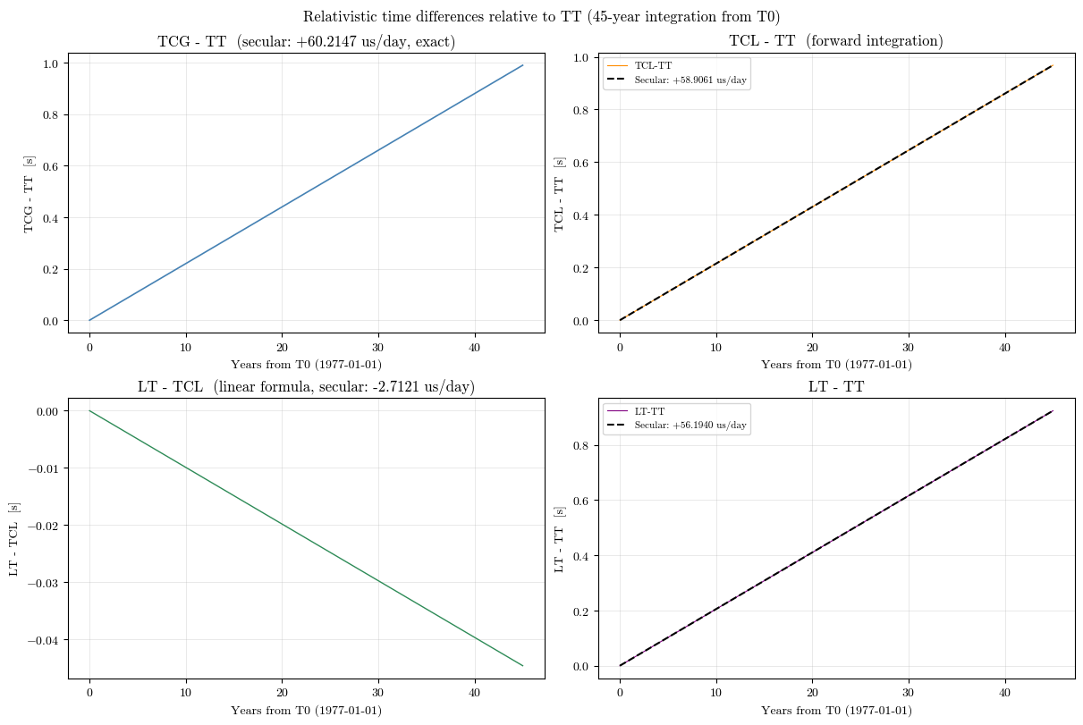
6. TCL-TCG comparison
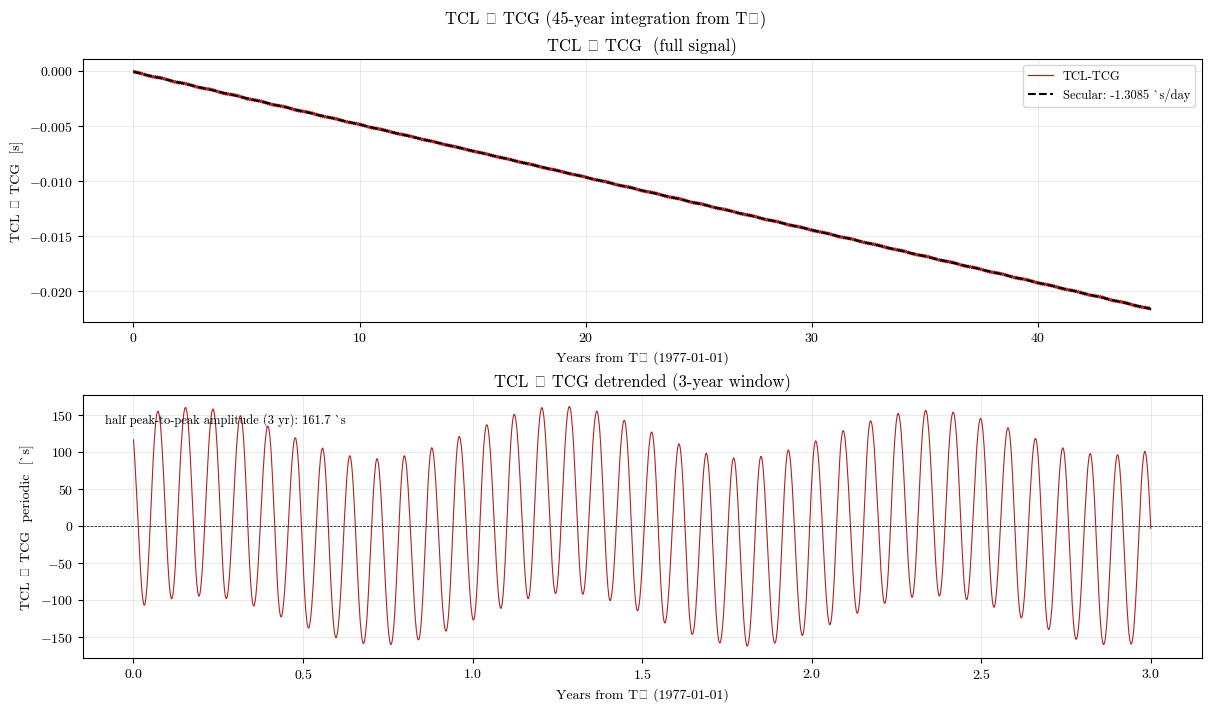
Because TCG-TT is exactly linear, the TCL-TCG curve is obtained by subtracting the TCG-TT line from TCL-TT:
The periodic terms are therefore inherited from TCL-TT, while the secular slope changes by the geocentric scaling rate.
[10]:
# TCL-TCG = (TCL-TT) - (TCG-TT),  where TCG-TT = rate_tcg_tt * days  (exact linear)
diff_tcl_tcg_us = diff_tcl_tt_us - diff_tcg_tt_us

# Secular rate of TCL-TCG
poly_tcl_tcg = np.polyfit(days, diff_tcl_tcg_us, 1)
trend_tcl_tcg = np.polyval(poly_tcl_tcg, days)
periodic_tcl_tcg = diff_tcl_tcg_us - trend_tcl_tcg

rate_tcl_tcg_num = poly_tcl_tcg[0]
print(f"TCL-TCG secular rate: {rate_tcl_tcg_num:+.4f} us/day")
print(f"  = TCL-TT ({poly_tcl[0]:+.4f}) - TCG-TT ({rate_tcg_tt:+.4f})")

# ---- Figure 1: 45-year time series ----
fig, axes = plt.subplots(2, 1, figsize=(12, 7), constrained_layout=True)
fig.suptitle("TCL – TCG (45-year integration from T₀)", fontsize=12)

ax = axes[0]
ax.plot(years, diff_tcl_tcg_us / 1e6, lw=0.9, color="firebrick", label="TCL-TCG")
ax.plot(
    years,
    trend_tcl_tcg / 1e6,
    lw=1.5,
    color="k",
    ls="--",
    label=f"Secular: {rate_tcl_tcg_num:+.4f} µs/day",
)
ax.set_ylabel("TCL – TCG  [s]")
ax.set_title("TCL – TCG  (full signal)")
ax.legend(fontsize=9)
ax.grid(True, lw=0.4, alpha=0.5)
ax.set_xlabel("Years from T₀ (1977-01-01)")

# ---- Figure 2: periodic terms (3-year zoom) ----
n_zoom3 = int(3 * 365.25 / dt_day) + 1
days_z3 = days[:n_zoom3]
years_z3 = days_z3 / 365.25
periodic_tcg_z = periodic_tcl_tcg[:n_zoom3]

ax = axes[1]
ax.plot(years_z3, periodic_tcg_z, lw=0.8, color="firebrick")
ax.axhline(0, color="k", lw=0.5, ls="--")
amp = (periodic_tcg_z.max() - periodic_tcg_z.min()) / 2
ax.text(
    0.02,
    0.93,
    f"half peak-to-peak amplitude (3 yr): {amp:.1f} µs",
    transform=ax.transAxes,
    fontsize=9,
    va="top",
)
ax.set_ylabel("TCL – TCG  periodic  [µs]")
ax.set_title("TCL – TCG detrended (3-year window)")
ax.set_xlabel("Years from T₀ (1977-01-01)")
ax.grid(True, lw=0.4, alpha=0.5)

plt.show()
TCL-TCG secular rate: -1.3085 us/day
  = TCL-TT (+58.9061) - TCG-TT (+60.2147)
/Users/keidaiiiyama/Documents/sw_navlab/LuPNT/.pixi/envs/default/lib/python3.11/site-packages/IPython/core/pylabtools.py:170: UserWarning: Glyph 8320 (\N{SUBSCRIPT ZERO}) missing from font(s) cmr10.
  fig.canvas.print_figure(bytes_io, **kw)
/Users/keidaiiiyama/Documents/sw_navlab/LuPNT/.pixi/envs/default/lib/python3.11/site-packages/IPython/core/pylabtools.py:170: UserWarning: Glyph 8211 (\N{EN DASH}) missing from font(s) cmr10.
  fig.canvas.print_figure(bytes_io, **kw)
[11]:
# FFT of TCL-TCG periodic terms (identical to TCL-TT since TCG-TT is linear)
N_tcg = n_zoom3
freqs_tcg = np.fft.rfftfreq(N_tcg, d=dt_day)
with np.errstate(divide="ignore"):
    periods_tcg = np.where(freqs_tcg > 0, 1.0 / freqs_tcg, np.inf)

amp_tcl_tcg = 2 * np.abs(np.fft.rfft(periodic_tcg_z[:N_tcg])) / N_tcg
mask_tcg = (periods_tcg >= 5) & (periods_tcg <= 500)

fig, ax = plt.subplots(figsize=(12, 4), constrained_layout=True)
ax.semilogy(periods_tcg[mask_tcg], amp_tcl_tcg[mask_tcg], lw=0.8, color="firebrick")
ax.set_ylabel("TCL – TCG  amplitude  [µs]")
ax.set_xlabel("Period  [days]")
ax.set_title("Amplitude spectrum of TCL – TCG periodic terms (3-year window)")
ax.set_xlim([5, 500])
ax.grid(True, which="both", lw=0.4, alpha=0.5)

ref_periods_tcg = {
    "Anomalistic\n27.56 d": 27.5545,
    "Sidereal\n27.32 d": 27.3217,
    "Synodic\n29.53 d": 29.5306,
    "Annual\n365.25 d": 365.25,
}
for lbl, per in ref_periods_tcg.items():
    idx = np.argmin(np.abs(periods_tcg - per))
    if mask_tcg[idx]:
        ax.axvline(per, color="k", lw=0.8, ls="--", alpha=0.6)
        ax.text(
            per,
            amp_tcl_tcg[mask_tcg].min(),
            lbl,
            ha="center",
            va="bottom",
            fontsize=7,
            alpha=0.9,
        )

plt.show()

# Top peaks in 20-40 day lunar month range
print("Dominant periodic components in TCL-TCG (20-40 day range):")
mask_lm = (periods_tcg >= 20) & (periods_tcg <= 40)
pk = np.argsort(amp_tcl_tcg[mask_lm])[::-1][:5]
for i, j in enumerate(pk):
    p = periods_tcg[mask_lm][j]
    a = amp_tcl_tcg[mask_lm][j]
    print(f"  {i+1}. Period = {p:.3f} days,  amplitude = {a:.4f} µs")

print()
print("Thesis reference (Sec. 4.2, Table 4.1):")
print("  Synodic  month (~29.53 d): dominant term (large amplitude)")
print("  Anomalistic month (27.56 d): 0.4778 µs  [Earth potential variation]")
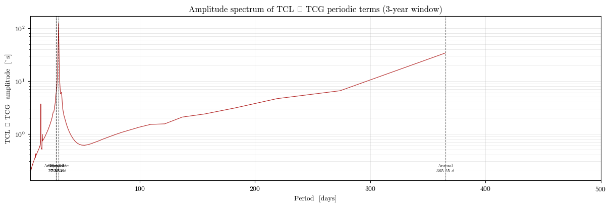
Dominant periodic components in TCL-TCG (20-40 day range):
  1. Period = 29.616 days,  amplitude = 123.5709 µs
  2. Period = 28.837 days,  amplitude = 15.3188 µs
  3. Period = 30.439 days,  amplitude = 11.5044 µs
  4. Period = 28.097 days,  amplitude = 7.3534 µs
  5. Period = 32.229 days,  amplitude = 6.1075 µs

Thesis reference (Sec. 4.2, Table 4.1):
  Synodic  month (~29.53 d): dominant term (large amplitude)
  Anomalistic month (27.56 d): 0.4778 µs  [Earth potential variation]
7. Periodic terms
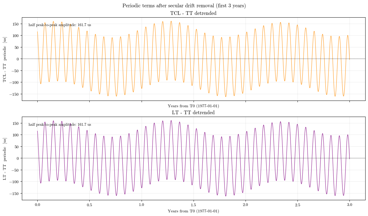
After removing a best-fit line, the residual shows the physical periodic signatures. The largest terms are associated with the Moon’s changing geometry with respect to the Sun and Earth: synodic-month, anomalistic-month, and annual variations.
This is the part of the time conversion that a simple constant drift cannot capture.
[12]:
# Show first 3 years for clarity
n_zoom = int(3 * 365.25 / dt_day) + 1
days_z = days[:n_zoom]
years_z = days_z / 365.25

# Detrend using the full-span secular rate (avoids end effects)
periodic_tcl_z = diff_tcl_tt_us[:n_zoom] - np.polyval(poly_tcl, days_z)
periodic_lt_z = diff_lt_tt_us[:n_zoom] - np.polyval(poly_lt_tt, days_z)

fig, axes = plt.subplots(2, 1, figsize=(12, 7), constrained_layout=True, sharex=True)
fig.suptitle("Periodic terms after secular drift removal (first 3 years)", fontsize=12)

ax = axes[0]
ax.plot(years_z, periodic_tcl_z, lw=0.8, color="darkorange")
ax.set_ylabel("TCL - TT  periodic  [us]")
ax.set_title("TCL - TT detrended")
ax.axhline(0, color="k", lw=0.5, ls="--")
amp_tcl = (periodic_tcl_z.max() - periodic_tcl_z.min()) / 2
ax.text(
    0.02,
    0.93,
    f"half peak-to-peak amplitude: {amp_tcl:.1f} us",
    transform=ax.transAxes,
    fontsize=9,
    va="top",
)

ax = axes[1]
ax.plot(years_z, periodic_lt_z, lw=0.8, color="purple")
ax.set_ylabel("LT - TT  periodic  [us]")
ax.set_title("LT - TT detrended")
ax.axhline(0, color="k", lw=0.5, ls="--")
amp_lt = (periodic_lt_z.max() - periodic_lt_z.min()) / 2
ax.text(
    0.02,
    0.93,
    f"half peak-to-peak amplitude: {amp_lt:.1f} us",
    transform=ax.transAxes,
    fontsize=9,
    va="top",
)

for ax in axes:
    ax.set_xlabel("Years from T0 (1977-01-01)")
    ax.grid(True, lw=0.4, alpha=0.5)

plt.show()
[13]:
# FFT analysis on the 3-year window
N = n_zoom
freqs = np.fft.rfftfreq(N, d=dt_day)  # cycles/day
with np.errstate(divide="ignore"):
    periods = np.where(freqs > 0, 1.0 / freqs, np.inf)  # days

amp_spec_tcl = 2 * np.abs(np.fft.rfft(periodic_tcl_z[:N])) / N  # us amplitude
amp_spec_lt = 2 * np.abs(np.fft.rfft(periodic_lt_z[:N])) / N

mask = (periods >= 5) & (periods <= 400)

ref_periods = {
    "Anomalistic\nmonth 27.56 d": 27.5545,
    "Sidereal\nmonth 27.32 d": 27.3217,
    "Synodic\nmonth 29.53 d": 29.5306,
    "Annual 365.25 d": 365.25,
}

fig, axes = plt.subplots(2, 1, figsize=(12, 7), constrained_layout=True)
fig.suptitle(
    "Amplitude spectrum of periodic terms in TCL-TT and LT-TT (3-year window)",
    fontsize=12,
)

for ax, spec, color, label in zip(
    axes,
    [amp_spec_tcl, amp_spec_lt],
    ["darkorange", "purple"],
    ["TCL - TT", "LT - TT"],
):
    ax.semilogy(periods[mask], spec[mask], lw=0.8, color=color)
    ax.set_ylabel(f"{label}  amplitude  [us]")
    ax.set_xlabel("Period  [days]")
    ax.set_xlim([5, 400])
    ax.grid(True, which="both", lw=0.4, alpha=0.5)
    for lbl, per in ref_periods.items():
        idx = np.argmin(np.abs(periods - per))
        if mask[idx]:
            ax.axvline(per, color="k", lw=0.8, ls="--", alpha=0.6)
            ax.text(
                per,
                ax.get_ylim()[0],
                lbl,
                ha="center",
                va="bottom",
                fontsize=7,
                alpha=0.9,
            )

plt.show()

# Print dominant peaks in lunar-month period range
print("Dominant periodic terms in TCL-TT (5-50 day range):")
mask_peaks = (periods >= 5) & (periods <= 50)
peak_idx = np.argsort(amp_spec_tcl[mask_peaks])[::-1][:6]
for i, idx in enumerate(peak_idx):
    p = periods[mask_peaks][idx]
    a = amp_spec_tcl[mask_peaks][idx]
    print(f"  {i+1}. Period = {p:.3f} days,  amplitude = {a:.4f} us")
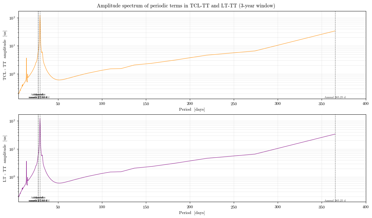
Dominant periodic terms in TCL-TT (5-50 day range):
  1. Period = 29.616 days,  amplitude = 123.5709 us
  2. Period = 28.837 days,  amplitude = 15.3188 us
  3. Period = 30.439 days,  amplitude = 11.5044 us
  4. Period = 28.097 days,  amplitude = 7.3534 us
  5. Period = 32.229 days,  amplitude = 6.1075 us
  6. Period = 31.309 days,  amplitude = 5.6765 us
8. Summary
This notebook used LuPNT time tools and a transparent Python reimplementation to show three lessons:
time scales are part of the navigation state model, not just formatting labels;
the LT-TT difference has both secular and periodic components;
LuPNT’s built-in conversion routines can be validated against the underlying relativistic integral when needed.
[14]:
print("Secular drift rate summary")
print("=" * 65)
print(f"{'Quantity':<20} {'Analytical [us/day]':<22} {'Numerical [us/day]':<20}")
print("-" * 65)
print(f"{'TCG - TT':<20} {rate_tcg_tt:+.4f}{'':<16} {'(exact linear)':>20}")
print(f"{'TCL - TT':<20} {'—':<22} {poly_tcl[0]:+.4f}")
print(f"{'LT  - TCL':<20} {rate_lt_tcl:+.4f}{'':<16} {poly_lt_tcl[0]:+.4f}")
print(f"{'LT  - TT':<20} {rate_lt_tt:+.4f}{'':<16} {poly_lt_tt[0]:+.4f}")
print("=" * 65)
Secular drift rate summary
=================================================================
Quantity             Analytical [us/day]    Numerical [us/day]
-----------------------------------------------------------------
TCG - TT             +60.2147                       (exact linear)
TCL - TT             —                      +58.9061
LT  - TCL            -2.7121                 -2.7121
LT  - TT             +56.0256                 +56.1940
=================================================================