Example 16: LEO PNT — a low-Earth-orbit navigation constellation
This is the Earth companion to the Mars tutorial (Example 15). Here we build a low-Earth-orbit (LEO) Position, Navigation and Timing constellation — the kind of dense small-satellite fleet proposed to augment GPS with strong, close-range signals — and evaluate the positioning service it delivers to a user in San Francisco.
LEO adds a force that higher orbits can ignore: atmospheric drag. LuPNT models it with a Harris-Priester density model, alongside the Earth gravity field, so the whole study runs on the native NBodyDynamics propagator and Earth reference frames.
We will
build an Earth force model with :math:`J_2` (and higher harmonics) plus atmospheric drag,
show that neglecting drag throws a LEO satellite’s predicted position off by kilometres within days — why a LEO PNT provider must model it,
lay out a 110-satellite Walker constellation at 600 km and propagate it,
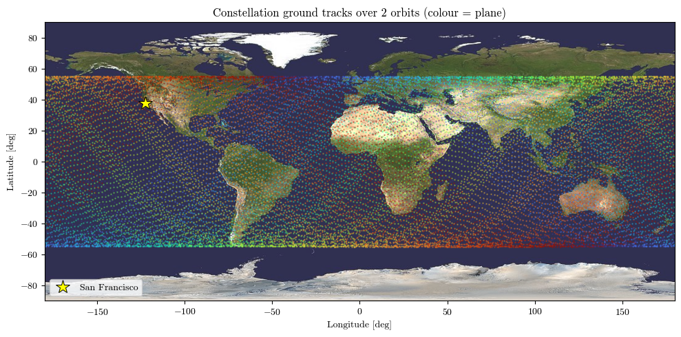
visualize the orbits and ground tracks,
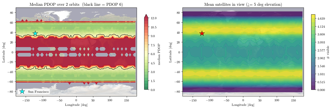
map coverage and PDOP over the surface, and
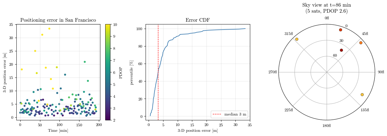
run a pseudorange least-squares positioning simulation at San Francisco.
Only the central body and its forces change from the lunar and Mars examples; the workflow is the same.
0. Imports and Earth data
Earth is a first-class body in LuPNT: Body.Earth gives its gravity model, GCRF / ITRF are the inertial and Earth-fixed frames, and plot_body already knows Earth’s texture.
[1]:
import os, sys
from pathlib import Path

import numpy as np
import matplotlib.pyplot as plt
import plotly.graph_objects as go
from PIL import Image

for _b in [Path.cwd(), *Path.cwd().parents]:
    if (_b / "python/pylupnt/__init__.py").exists():
        sys.path.insert(0, str((_b / "python").resolve()))
        if (_b / "data/LuPNT_data/ephemeris").is_dir():
            os.environ["LUPNT_DATA_PATH"] = str((_b / "data/LuPNT_data").resolve())
        break
import pylupnt as pnt

np.set_printoptions(precision=4, suppress=True)
RAD, DEG = pnt.RAD, pnt.DEG
LUPNT_DATA = os.environ["LUPNT_DATA_PATH"]

earth_pm = pnt.Body.Earth()
GM_EARTH = float(earth_pm.GM)  # [m^3/s^2]
R_EARTH = float(earth_pm.R)  # [m]
EARTH_MAP = np.asarray(
    Image.open(os.path.join(LUPNT_DATA, "topo", "earth_surface.jpg"))
)
EARTH_MAP = np.fliplr(
    np.flipud(EARTH_MAP)
)  # flip to match the coordinate system of the Earth-fixed frame

print(f"GM_EARTH = {GM_EARTH:.6e} m^3/s^2")
print(f"R_EARTH  = {R_EARTH/1e3:.1f} km")
print(
    f"frames   : {earth_pm.inertial_frame} (inertial) / {earth_pm.fixed_frame} (Earth-fixed)"
)

# Host heavy interactive figures on lupnt-doc-assets instead of embedding them.
import sys as _sys
from pathlib import Path as _Path

for _p in [_Path.cwd(), *_Path.cwd().parents]:
    if (_p / "python" / "examples" / "_doc_assets.py").exists():
        _sys.path.insert(0, str(_p / "python" / "examples"))
        break
from _doc_assets import embed_plotly, embed_cesium_scene
[00.00][PyLuPNT] Initializing
GM_EARTH = 3.986004e+14 m^3/s^2
R_EARTH  = 6378.1 km
frames   : Frame.GCRF (inertial) / Frame.ITRF (Earth-fixed)
1. Force model: \(J_2\) gravity and atmospheric drag
Body.Earth(n, m, gravity_file) loads the EGM96 field (we keep degree/order \(4\times4\) — \(J_2\) dominates the low-orbit dynamics). We then switch on atmospheric drag with set_drag_coeff, which sets the ballistic coefficient \(B = C_D A/m\); LuPNT evaluates the drag with a Harris-Priester density model (valid 100–1000 km) that needs no extra data.
compute_accelerations(..., decompose_gravity=True) shows the resulting budget: \(J_2\) is four orders of magnitude below the central term, and drag is another few orders below that — but drag is the one force here that removes energy, so its effect accumulates secularly.
[2]:
N_GRAV = 4  # EGM96 degree/order (J2-dominated for LEO)
CD, AREA, MASS = 2.2, 1.0, 100.0  # drag coefficient, area [m^2], mass [kg]
BSTAR = CD * AREA / MASS  # ballistic coefficient B = CD*A/m [m^2/kg]

earth = pnt.Body.Earth(N_GRAV, N_GRAV, gravity_file="EGM96.cof")
GCRF, ITRF = earth.inertial_frame, earth.fixed_frame


def make_dynamics(drag=True, integrator=pnt.IntegratorType.RK4, step=30.0):
    dyn = pnt.NBodyDynamics()
    dyn.set_frame(GCRF)
    dyn.set_units(pnt.SI_UNITS)
    dyn.add_body(earth)  # Earth gravity field (incl. J2)
    dyn.set_integrator(integrator)
    dyn.set_time_step(step)
    if drag:
        dyn.set_drag_coeff(BSTAR)  # Harris-Priester atmospheric drag
    return dyn


dyn = make_dynamics(drag=True)
EPOCH = pnt.gregorian_to_time(2035, 1, 1, 0, 0, 0)

# acceleration budget at three LEO altitudes (circular, 55 deg)
print(f"Ballistic coefficient B = CD*A/m = {BSTAR:.3f} m^2/kg\n")
print(f"{'altitude':>10} {'|a_grav|':>12} {'|a_J2|':>12} {'|a_drag|':>12}")
for alt in (400e3, 600e3, 800e3):
    rv = pnt.classical_to_cart(
        np.array([R_EARTH + alt, 0.001, 55 * RAD, 0, 0, 0]), GM_EARTH
    )
    acc = dyn.compute_accelerations(EPOCH, rv, decompose_gravity=True)
    m = {k: float(np.linalg.norm(v)) for k, v in acc.items()}
    print(
        f"{alt/1e3:>7.0f} km {m['EARTH_gravity']:>12.4e} {m.get('EARTH_J2',0):>12.3e} "
        f"{m.get('drag',0):>12.3e}"
    )
Ballistic coefficient B = CD*A/m = 0.022 m^2/kg

  altitude     |a_grav|       |a_J2|     |a_drag|
    400 km   8.6933e+00    1.253e-02    3.277e-06
    600 km   8.2022e+00    1.115e-02    2.299e-07
    800 km   7.7515e+00    9.958e-03    2.683e-08
2. Why drag matters for a LEO PNT provider
A navigation satellite broadcasts its own predicted position; any error there flows straight into the user’s fix. To show what drag does, we propagate one satellite at the constellation altitude twice — with and without drag — from the same initial state, and track how far apart the two predictions drift. Because both runs use the same accurate integrator (RK8), numerical error cancels in the difference, isolating the drag effect: an unmodeled satellite falls behind along-track and its position error grows to hundreds of metres to kilometres within days — unacceptable for PNT.
[3]:
ALT_DEMO = 600e3
rv_demo = pnt.classical_to_cart(
    np.array([R_EARTH + ALT_DEMO, 0.0005, 55 * RAD, 0, 0, 0]), GM_EARTH
)
t_demo = EPOCH + np.arange(0.0, 5 * 86400.0, 900.0)  # 5 days, 15-min samples

dyn_drag = make_dynamics(drag=True, integrator=pnt.IntegratorType.RK8, step=60.0)
dyn_nodrag = make_dynamics(drag=False, integrator=pnt.IntegratorType.RK8, step=60.0)
xd = np.asarray(dyn_drag.propagate(rv_demo, t_demo))
xn = np.asarray(dyn_nodrag.propagate(rv_demo, t_demo))
sep = np.linalg.norm(xd[:, :3] - xn[:, :3], axis=1)  # drag-induced position error [m]
days = (t_demo - EPOCH) / 86400.0

fig, ax = plt.subplots(figsize=(7.5, 4.0))
ax.plot(days, sep / 1e3, color="crimson", lw=1.6)
ax.set_xlabel("Time [days]")
ax.set_ylabel("Position error from ignoring drag [km]")
ax.set_title(
    f"Unmodeled-drag ephemeris error at {ALT_DEMO/1e3:.0f} km (B = {BSTAR:.3f} m$^2$/kg)"
)
ax.grid(alpha=0.3)
plt.tight_layout()
plt.show()
print(
    f"Neglecting drag mispredicts the satellite by {sep[-1]/1e3:.2f} km after {days[-1]:.0f} days."
)
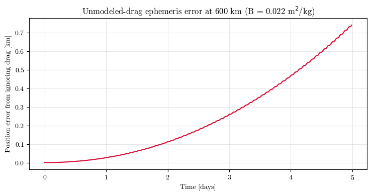
Neglecting drag mispredicts the satellite by 0.74 km after 5 days.
3. A 110-satellite Walker constellation
We use a Walker :math:`delta` pattern \(110/10/1\): 110 satellites in 10 planes, circular orbits at 600 km and :math:`55^circ` inclination — enough to give a mid-latitude user like San Francisco continuous multi-satellite visibility.
Unlike Mars (Example 15), Earth needs no special design frame: GCRF’s pole sits within a fraction of a degree of Earth’s spin axis, so an inclination specified in GCRF is the geographic inclination to well within our purposes. We build each satellite’s state with classical_to_cart directly in GCRF.
[4]:
N_SAT, N_PLANES, F_WALKER = 110, 10, 1
SATS_PER_PLANE = N_SAT // N_PLANES
ALT = 600e3
A_SMA = R_EARTH + ALT
INC = 55.0 * RAD
PERIOD = 2 * np.pi * np.sqrt(A_SMA**3 / GM_EARTH)


def walker_elements(T, P, Fp, a, e, inc):
    spp = T // P
    coes = []
    for p in range(P):
        raan = p * 2 * np.pi / P
        for s in range(spp):
            M = (s * 2 * np.pi / spp + p * 2 * np.pi * Fp / T) % (2 * np.pi)
            coes.append([a, e, inc, raan, 0.0, M])
    return np.array(coes)


COES = walker_elements(N_SAT, N_PLANES, F_WALKER, A_SMA, 0.001, INC)
RV0 = np.array([pnt.classical_to_cart(coe, GM_EARTH) for coe in COES])  # GCRF states

print(
    f"Walker {N_SAT}/{N_PLANES}/{F_WALKER}: {N_PLANES} planes x {SATS_PER_PLANE} sats"
)
print(
    f"  altitude {ALT/1e3:.0f} km  (a = {A_SMA/1e3:.0f} km),  inclination {INC*DEG:.0f} deg"
)
print(f"  orbital period {PERIOD/60:.1f} min  ({86400/PERIOD:.1f} revs/day)")
Walker 110/10/1: 10 planes x 11 sats
  altitude 600 km  (a = 6978 km),  inclination 55 deg
  orbital period 96.7 min  (14.9 revs/day)
Propagate the fleet with \(J_2\) + drag
We propagate all 110 satellites for two orbital periods at 1-minute sampling with NBodyDynamics (fixed-step RK4 — more than accurate enough for coverage geometry), then rotate the inertial GCRF states into the Earth-fixed ITRF frame with convert_frame for ground tracks and user geometry.
[5]:
T_SIM = 2 * PERIOD
DT = 60.0
TS = EPOCH + np.arange(0.0, T_SIM, DT)
N_T = len(TS)

POS_GCRF = np.zeros((N_SAT, N_T, 3))
for k in range(N_SAT):
    POS_GCRF[k] = np.asarray(dyn.propagate(RV0[k], TS))[:, :3]

POS_ITRF = np.zeros((N_SAT, N_T, 3))
for k in range(N_SAT):
    POS_ITRF[k] = np.asarray(pnt.convert_frame(TS, POS_GCRF[k], GCRF, ITRF))[:, :3]

print(
    f"Propagated {N_SAT} satellites over {T_SIM/60:.0f} min ({N_T} epochs) with J2 + drag"
)
Propagated 110 satellites over 193 min (194 epochs) with J2 + drag
4. The constellation in 3-D
plot_body draws the textured Earth and plot_orbits the trajectories (colour = orbital plane).
[6]:
n_one = int(np.ceil(PERIOD / DT))
plane_colors = plt.cm.turbo(np.linspace(0.05, 0.95, N_PLANES))
plane_hex = [
    "#%02x%02x%02x" % tuple(int(255 * c) for c in col[:3]) for col in plane_colors
]

fig = go.Figure()
# finer sphere + richer colours than the defaults (the Earth texture is 512x1024)
pnt.plot.plot_body(fig, pnt.EARTH, size_factor=2, n_colors=96, n_training_pixels=40000)
for k in range(N_SAT):
    pnt.plot.plot_orbits(fig, POS_GCRF[k, :n_one], color=plane_hex[k // SATS_PER_PLANE])
fig.add_scatter3d(
    x=POS_GCRF[:, 0, 0] / 1e6,
    y=POS_GCRF[:, 0, 1] / 1e6,
    z=POS_GCRF[:, 0, 2] / 1e6,
    mode="markers",
    marker=dict(size=2.5, color="black"),
    name="satellites",
)
pnt.plot.set_view(fig, azimuth=30, elevation=25, zoom=2.4)
fig.update_layout(
    width=640,
    height=640,
    title=f"LEO PNT Walker {N_SAT}/{N_PLANES}/{F_WALKER} at {ALT/1e3:.0f} km (GCRF)",
)
embed_plotly(fig, "ex16_leopnt")
[doc-asset] plots/ex16_leopnt.html (12546 kB) -> https://stanford-navlab.github.io/lupnt-doc-assets/plots/ex16_leopnt.html
5. Ground tracks
In the Earth-fixed frame the tracks slide westward as Earth rotates under the orbits, sweeping the whole \(\pm55^\circ\) latitude band over a couple of hours.
[7]:
lla = np.array(
    [np.asarray(pnt.cart_to_lat_lon_alt(POS_ITRF[k], R_EARTH)) for k in range(N_SAT)]
)

fig, ax = plt.subplots(figsize=(10, 5))
ax.imshow(
    EARTH_MAP, extent=[-180, 180, -90, 90], aspect="auto", origin="upper", alpha=0.85
)
for k in range(N_SAT):
    lon = ((lla[k, :, 1] + 180.0) % 360.0) - 180.0
    ax.scatter(
        lon, lla[k, :, 0], s=0.6, color=plane_hex[k // SATS_PER_PLANE], alpha=0.4
    )
ax.plot(
    -122.42, 37.77, "*", ms=15, color="yellow", mec="k", mew=0.7, label="San Francisco"
)
ax.set_xlim(-180, 180)
ax.set_ylim(-90, 90)
ax.set_xlabel("Longitude [deg]")
ax.set_ylabel("Latitude [deg]")
ax.set_title("Constellation ground tracks over 2 orbits (colour = plane)")
ax.legend(loc="lower left")
plt.tight_layout()
plt.show()
6. Coverage and PDOP
With line-of-sight unit vectors \(\hat{\mathbf u}_i\) (local East-North-Up) to the visible satellites, the geometry matrix stacks rows \([\hat u_E,\hat u_N,\hat u_U,1]\) and
We map the median PDOP over the two-orbit window on a \(4^\circ\) grid. A \(55^\circ\)-inclination LEO fleet serves a broad mid-latitude band well (San Francisco included) and thins out toward the poles — the characteristic footprint of an inclined Walker constellation.
[8]:
MASK_DEG = 5.0
MASK = np.deg2rad(MASK_DEG)
SF = (37.7749, -122.4194)  # San Francisco (lat N, lon E)


def pdop_stack(u_enu, visible):
    H = np.concatenate([u_enu, np.ones(u_enu.shape[:-1] + (1,))], axis=-1)
    Hw = H * visible[..., None]
    M = np.einsum("...sa,...sb->...ab", Hw, H)
    bad = visible.sum(axis=-1) < 4
    M[bad] = np.eye(4)
    Minv = np.linalg.inv(M)
    pdop = np.sqrt(
        np.clip(Minv[..., 0, 0] + Minv[..., 1, 1] + Minv[..., 2, 2], 0.0, None)
    )
    pdop[bad] = np.nan
    return pdop


LAT_G = np.arange(-82.0, 82.1, 4.0)
LON_G = np.arange(-180.0, 180.0, 4.0)
sub = slice(0, N_T, 2)  # subsample time to keep the map fast
PF = POS_ITRF[:, sub, :]
med_pdop = np.full((len(LAT_G), len(LON_G)), np.nan)
mean_vis = np.zeros_like(med_pdop)

for i, la in enumerate(np.deg2rad(LAT_G)):
    lo = np.deg2rad(LON_G)
    E = np.stack([-np.sin(lo), np.cos(lo), np.zeros_like(lo)], -1)
    Nn = np.stack(
        [
            -np.sin(la) * np.cos(lo),
            -np.sin(la) * np.sin(lo),
            np.full_like(lo, np.cos(la)),
        ],
        -1,
    )
    Up = np.stack(
        [
            np.cos(la) * np.cos(lo),
            np.cos(la) * np.sin(lo),
            np.full_like(lo, np.sin(la)),
        ],
        -1,
    )
    ru = R_EARTH * Up
    los = PF[None, :, :, :] - ru[:, None, None, :]
    e = np.einsum("lc,lstc->lst", E, los)
    n = np.einsum("lc,lstc->lst", Nn, los)
    u = np.einsum("lc,lstc->lst", Up, los)
    rng = np.sqrt(e**2 + n**2 + u**2)
    vis = np.arcsin(np.clip(u / rng, -1, 1)) >= MASK
    u_enu = np.moveaxis(np.stack([e / rng, n / rng, u / rng], -1), 1, 2)
    pdop = pdop_stack(u_enu, np.moveaxis(vis, 1, 2))
    covered = ~np.all(np.isnan(pdop), axis=1)  # cells that ever see >= 4 sats
    med_pdop[i, covered] = np.nanmedian(
        pdop[covered], axis=1
    )  # leave uncovered cells NaN
    mean_vis[i] = vis.sum(1).mean(1)

band = np.abs(LAT_G) <= 60
print(
    f"Median PDOP over the |lat|<=60 deg service band : {np.nanmedian(med_pdop[band]):.2f}"
)
print(f"Mean satellites in view (that band)             : {mean_vis[band].mean():.2f}")
Median PDOP over the |lat|<=60 deg service band : 6.65
Mean satellites in view (that band)             : 3.50
[9]:
fig, axes = plt.subplots(1, 2, figsize=(14, 4.6))

ax = axes[0]
ax.imshow(
    EARTH_MAP, extent=[-180, 180, -90, 90], aspect="auto", origin="upper", alpha=0.35
)
cf = ax.contourf(
    LON_G,
    LAT_G,
    np.clip(med_pdop, 0, 12),
    levels=np.linspace(0, 12, 25),
    cmap="RdYlGn_r",
    alpha=0.8,
    extend="max",
)
ax.contour(
    LON_G, LAT_G, np.clip(med_pdop, 0, 12), levels=[6], colors="k", linewidths=1.0
)
ax.plot(SF[1], SF[0], "*", ms=16, color="cyan", mec="k", mew=0.6, label="San Francisco")
ax.set_title("Median PDOP over 2 orbits  (black line = PDOP 6)")
ax.set_xlabel("Longitude [deg]")
ax.set_ylabel("Latitude [deg]")
ax.legend(loc="lower left")
plt.colorbar(cf, ax=ax, label="median PDOP", shrink=0.85)

ax = axes[1]
ax.imshow(
    EARTH_MAP, extent=[-180, 180, -90, 90], aspect="auto", origin="upper", alpha=0.35
)
cf2 = ax.contourf(
    LON_G,
    LAT_G,
    mean_vis,
    levels=np.linspace(0, mean_vis.max(), 20),
    cmap="viridis",
    alpha=0.8,
)
ax.plot(SF[1], SF[0], "*", ms=16, color="red", mec="k", mew=0.6)
ax.set_title("Mean satellites in view (>= 5 deg elevation)")
ax.set_xlabel("Longitude [deg]")
ax.set_ylabel("Latitude [deg]")
plt.colorbar(cf2, ax=ax, label="# visible", shrink=0.85)

plt.tight_layout()
plt.show()
7. User positioning in San Francisco
Finally, the user experience. At San Francisco (\(37.77^\circ\)N, \(122.42^\circ\)W) we form a pseudorange to every visible satellite,
with a receiver clock bias \(c\,\delta t\) and \(\sigma=1\) m ranging noise, and solve for position and clock by iterated least squares whenever four or more satellites are in view. (LEO satellites sit close overhead, so we seed the solver at a coarse surface point beneath the visible set rather than at Earth’s centre.)
[10]:
def enu_basis(lat, lon):
    cl, sl, co, so = np.cos(lat), np.sin(lat), np.cos(lon), np.sin(lon)
    return np.array([[-so, co, 0.0], [-sl * co, -sl * so, cl], [cl * co, cl * so, sl]])


lat_u, lon_u = np.deg2rad(SF[0]), np.deg2rad(SF[1])
r_user = R_EARTH * np.array(
    [np.cos(lat_u) * np.cos(lon_u), np.cos(lat_u) * np.sin(lon_u), np.sin(lat_u)]
)
Renu = enu_basis(lat_u, lon_u)

los = POS_ITRF - r_user[None, None, :]
enu = np.einsum("ij,ktj->kti", Renu, los)
rng_u = np.linalg.norm(enu, axis=-1)
elev_u = np.arcsin(np.clip(enu[..., 2] / rng_u, -1, 1))
az_u = np.arctan2(enu[..., 0], enu[..., 1])
vis_u = elev_u >= MASK

SIGMA = 1.0
rng_gen = np.random.default_rng(0)
err3d, err_h, err_v, epochs_fix, pdop_fix, nvis_fix = [], [], [], [], [], []
n_visible = vis_u.sum(0)

for tt in range(N_T):
    m = vis_u[:, tt]
    if m.sum() < 4:
        continue
    sats = POS_ITRF[m, tt, :]
    rho = (
        np.linalg.norm(sats - r_user, axis=1) + rng_gen.standard_normal(m.sum()) * SIGMA
    )
    x = np.concatenate([R_EARTH * (sats.mean(0) / np.linalg.norm(sats.mean(0))), [0.0]])
    converged = False
    for _ in range(20):
        d = x[:3] - sats
        r = np.linalg.norm(d, axis=1)
        H = np.concatenate([d / r[:, None], np.ones((m.sum(), 1))], axis=1)
        dx = np.linalg.lstsq(H, rho - (r + x[3]), rcond=None)[0]
        x += dx
        if np.linalg.norm(dx[:3]) < 1e-3:
            converged = True
            break
    if not converged or abs(np.linalg.norm(x[:3]) - R_EARTH) > 5e5:
        continue  # drop degenerate / divergent geometries
    derr = Renu @ (x[:3] - r_user)
    err3d.append(np.linalg.norm(derr))
    err_h.append(np.hypot(derr[0], derr[1]))
    err_v.append(abs(derr[2]))
    epochs_fix.append((TS[tt] - EPOCH) / 60.0)
    Q = np.linalg.inv(H.T @ H)
    pdop_fix.append(np.sqrt(Q[0, 0] + Q[1, 1] + Q[2, 2]))
    nvis_fix.append(int(m.sum()))

err3d = np.array(err3d)
err_h = np.array(err_h)
err_v = np.array(err_v)
pdop_fix = np.array(pdop_fix)
epochs_fix = np.array(epochs_fix)

print(
    f"Satellites in view at SF : min {n_visible.min()}, mean {n_visible.mean():.1f}, "
    f"max {n_visible.max()}"
)
print(f"Epochs with a fix        : {len(err3d)} / {N_T} ({100*len(err3d)/N_T:.0f}%)")
print(
    f"3-D position error   median {np.median(err3d):6.1f} m   95% {np.percentile(err3d,95):6.1f} m"
)
print(f"  horizontal         median {np.median(err_h):6.1f} m")
print(f"  vertical           median {np.median(err_v):6.1f} m")
print(f"PDOP at fix epochs    median {np.median(pdop_fix):.2f}")
Satellites in view at SF : min 2, mean 4.5, max 6
Epochs with a fix        : 166 / 194 (86%)
3-D position error   median    3.3 m   95%   15.6 m
  horizontal         median    1.3 m
  vertical           median    2.9 m
PDOP at fix epochs    median 4.94
[11]:
fig = plt.figure(figsize=(13, 4.4))

ax = fig.add_subplot(1, 3, 1)
sc = ax.scatter(epochs_fix, err3d, c=pdop_fix, cmap="viridis", s=14, vmin=2, vmax=10)
ax.set_xlabel("Time [min]")
ax.set_ylabel("3-D position error [m]")
ax.set_title("Positioning error in San Francisco")
ax.grid(alpha=0.3)
plt.colorbar(sc, ax=ax, label="PDOP")

ax = fig.add_subplot(1, 3, 2)
xs = np.sort(err3d)
ys = np.arange(1, len(xs) + 1) / len(xs)
ax.plot(xs, ys * 100, color="steelblue")
ax.axvline(
    np.median(err3d),
    color="red",
    ls="--",
    lw=1,
    label=f"median {np.median(err3d):.0f} m",
)
ax.set_xlabel("3-D position error [m]")
ax.set_ylabel("percentile [%]")
ax.set_title("Error CDF")
ax.grid(alpha=0.3)
ax.legend()

ax = fig.add_subplot(1, 3, 3, projection="polar")
best = np.argmin(pdop_fix)
tt = int(round(epochs_fix[best] * 60.0 / DT))
m = vis_u[:, tt]
ax.set_theta_zero_location("N")
ax.set_theta_direction(-1)
ax.scatter(
    az_u[m, tt],
    90 - np.rad2deg(elev_u[m, tt]),
    c=[plane_hex[k // SATS_PER_PLANE] for k in np.where(m)[0]],
    s=45,
    edgecolors="k",
    lw=0.4,
)
ax.set_rmax(90)
ax.set_rticks([30, 60, 90])
ax.set_yticklabels(["60", "30", "0"])
ax.set_title(
    f"Sky view at t={epochs_fix[best]:.0f} min\n({m.sum()} sats, PDOP {pdop_fix[best]:.1f})",
    va="bottom",
)

plt.tight_layout()
plt.show()
8. On-board orbit determination (ODTS) with GPS
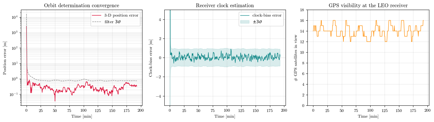
There is a flip side to the service above: before a LEO PNT satellite can broadcast its position, it has to know it. Each satellite carries its own GPS receiver and runs an on-board orbit- and time-determination (ODTS) filter — from ~600 km it looks up at the GPS constellation (~20,200 km) and sees most of it at once. This is also where drag comes back: the on-board filter uses a cheap gravity-only dynamics model and lets the GPS measurements plus process noise soak up the unmodeled drag.
We estimate the state \(\mathbf x = [\mathbf r,\ \mathbf v,\ b,\ d]\) — position, velocity, receiver clock bias \(b\) and drift \(d\) — with an Extended Kalman Filter:
predict — the orbit is propagated with
NBodyDynamics, whosepropagate_stm_with_inforeturns both the state and the \(6\times6\) state-transition matrix for the covariance; the clock uses \(b\leftarrow b + d\,\Delta t\);update — each visible GPS satellite gives an iono-free pseudorange \(\rho = \lVert\mathbf r_\text{GPS}-\mathbf r\rVert + b + \varepsilon\) (\(\sigma=1\) m), with measurement row \([-\hat{\mathbf e}^{\top},\,\mathbf 0^{\top},\,1,\,0]\).
We first build a nominal GPS constellation to range against.
[12]:
# nominal GPS: Walker 24/6/2, ~20,200 km, 55 deg -- stable MEO, propagated two-body (truth)
GPS_COES = walker_elements(24, 6, 2, R_EARTH + 20200e3, 0.0, 55.0 * RAD)
gps_dyn = pnt.CartesianTwoBodyDynamics(GM_EARTH)

DT_ODTS = 30.0  # measurement cadence [s]
TS_ODTS = EPOCH + np.arange(0.0, 2 * PERIOD, DT_ODTS)
N_ODTS = len(TS_ODTS)

# Truth: LEO nav-satellite 0 propagated WITH drag, and the GPS satellites.
leo_truth = np.asarray(dyn.propagate(RV0[0], TS_ODTS))  # (N,6): [r, v] in GCRF
gps_truth = np.array(
    [
        np.asarray(gps_dyn.propagate(pnt.classical_to_cart(c, GM_EARTH), TS_ODTS))[
            :, :3
        ]
        for c in GPS_COES
    ]
)  # (24,N,3)


def gps_visible(r_leo, r_gps, r_occ):
    """True if the LEO->GPS line of sight clears the Earth (occulting radius r_occ)."""
    d = r_gps - r_leo
    L = np.linalg.norm(d)
    u = d / L
    s = -np.dot(r_leo, u)  # foot of perpendicular from Earth centre
    if s < 0 or s > L:
        return True
    return np.linalg.norm(r_leo + s * u) > r_occ


R_OCC = R_EARTH + 50e3
n_gps_view = np.array(
    [
        sum(gps_visible(leo_truth[k, :3], gps_truth[j, k], R_OCC) for j in range(24))
        for k in range(N_ODTS)
    ]
)
print(
    f"GPS satellites in view from the LEO receiver: "
    f"min {n_gps_view.min()}, mean {n_gps_view.mean():.1f}, max {n_gps_view.max()}"
)
GPS satellites in view from the LEO receiver: min 12, mean 14.0, max 16
Run the Extended Kalman Filter
The truth orbit includes drag; the filter’s dynamics model does not — that mismatch is what the process noise Q_ACC represents. We start the filter 2 km and 2 m/s off with a wrong clock, and let GPS pull it in.
[13]:
dyn_filter = make_dynamics(drag=False)  # on-board model: gravity only (drag unmodeled)

SIGMA_RHO = 1.0  # iono-free pseudorange noise [m]
Q_ACC = 1e-5  # dynamics process noise (accel) [m/s^2]
Q_CLK = 5e-4  # clock-drift random walk [m/s/sqrt(s)]

# Truth receiver clock: bias b [m] and drift d [m/s] (slowly wandering).
rng = np.random.default_rng(1)
b_true = np.zeros(N_ODTS)
d_true = np.zeros(N_ODTS)
b_true[0], d_true[0] = 30.0, 0.20
for k in range(1, N_ODTS):
    d_true[k] = d_true[k - 1] + rng.standard_normal() * 1e-4 * np.sqrt(DT_ODTS)
    b_true[k] = b_true[k - 1] + d_true[k - 1] * DT_ODTS

# Initial estimate: truth + gross errors.
x = np.concatenate([RV0[0].astype(float), [b_true[0] + 80.0, d_true[0] + 0.4]])
x[:3] += rng.standard_normal(3) * 2000.0  # 2 km position error
x[3:6] += rng.standard_normal(3) * 2.0  # 2 m/s velocity error
P = np.diag([3e3**2] * 3 + [3.0] * 3 + [300.0**2, 1.0**2])

pos_err, pos_3sig, clk_err, clk_3sig = [], [], [], []
for k in range(N_ODTS):
    if k > 0:
        # --- predict: native STM for the orbit, analytic model for the clock ---
        xf, stm, _ = dyn_filter.propagate_stm_with_info(
            x[:6], TS_ODTS[k - 1], TS_ODTS[k]
        )
        x[:6] = np.asarray(xf)
        x[6] += x[7] * DT_ODTS
        Phi = np.eye(8)
        Phi[:6, :6] = np.asarray(stm)
        Phi[6, 7] = DT_ODTS
        Q = np.zeros((8, 8))
        Q[0:3, 0:3] = np.eye(3) * Q_ACC**2 * DT_ODTS**3 / 3
        Q[0:3, 3:6] = np.eye(3) * Q_ACC**2 * DT_ODTS**2 / 2
        Q[3:6, 0:3] = Q[0:3, 3:6].T
        Q[3:6, 3:6] = np.eye(3) * Q_ACC**2 * DT_ODTS
        Q[6, 6] = Q_CLK**2 * DT_ODTS**3 / 3
        Q[7, 7] = Q_CLK**2 * DT_ODTS
        P = Phi @ P @ Phi.T + Q

    # a-priori errors (current estimate before this epoch's measurements)
    pos_err.append(np.linalg.norm(x[:3] - leo_truth[k, :3]))
    pos_3sig.append(3 * np.sqrt(P[0, 0] + P[1, 1] + P[2, 2]))
    clk_err.append(x[6] - b_true[k])
    clk_3sig.append(3 * np.sqrt(P[6, 6]))

    # --- update: one pseudorange per visible GPS satellite ---
    r_leo = leo_truth[k, :3]
    vis = [j for j in range(24) if gps_visible(r_leo, gps_truth[j, k], R_OCC)]
    H = np.zeros((len(vis), 8))
    y = np.zeros(len(vis))
    for i, j in enumerate(vis):
        r_gps = gps_truth[j, k]
        rho = (
            np.linalg.norm(r_gps - r_leo)
            + b_true[k]
            + rng.standard_normal() * SIGMA_RHO
        )
        rho_pred = np.linalg.norm(r_gps - x[:3])
        H[i, :3] = -(r_gps - x[:3]) / rho_pred  # d(range)/d(r)
        H[i, 6] = 1.0  # d(range)/d(clock bias)
        y[i] = rho - (rho_pred + x[6])
    K = P @ H.T @ np.linalg.inv(H @ P @ H.T + np.eye(len(vis)) * SIGMA_RHO**2)
    x = x + K @ y
    P = (np.eye(8) - K @ H) @ P

pos_err = np.array(pos_err)
pos_3sig = np.array(pos_3sig)
clk_err = np.array(clk_err)
clk_3sig = np.array(clk_3sig)
t_min = (TS_ODTS - EPOCH) / 60.0
half = N_ODTS // 2
print(
    f"Position: initial error {pos_err[0]/1e3:.2f} km  ->  steady-state RMS "
    f"{np.sqrt(np.mean(pos_err[half:] ** 2)):.2f} m"
)
print(
    f"Clock bias: steady-state estimation error RMS {np.sqrt(np.mean(clk_err[half:] ** 2)):.2f} m "
    f"({np.sqrt(np.mean(clk_err[half:] ** 2))/299792458.0*1e9:.2f} ns)"
)
print(
    f"Filter consistency: {100*np.mean(pos_err[half:] < pos_3sig[half:]):.0f}% of steady-state "
    f"epochs have |error| < 3-sigma"
)
Position: initial error 2.56 km  ->  steady-state RMS 0.32 m
Clock bias: steady-state estimation error RMS 0.24 m (0.79 ns)
Filter consistency: 100% of steady-state epochs have |error| < 3-sigma
[14]:
fig, axes = plt.subplots(1, 3, figsize=(14, 4.0))

ax = axes[0]
ax.semilogy(t_min, pos_err, color="crimson", lw=1.2, label="3-D position error")
ax.semilogy(t_min, pos_3sig, color="gray", lw=1.0, ls="--", label=r"filter $3\sigma$")
ax.set_xlabel("Time [min]")
ax.set_ylabel("Position error [m]")
ax.set_title("Orbit determination convergence")
ax.grid(alpha=0.3, which="both")
ax.legend()

ax = axes[1]
ax.plot(t_min, clk_err, color="teal", lw=1.0, label="clock-bias error")
ax.fill_between(
    t_min, -clk_3sig, clk_3sig, color="teal", alpha=0.15, label=r"$\pm3\sigma$"
)
ax.set_xlabel("Time [min]")
ax.set_ylabel("Clock-bias error [m]")
ax.set_ylim(-5, 5)
ax.set_title("Receiver clock estimation")
ax.grid(alpha=0.3)
ax.legend()

ax = axes[2]
ax.plot(t_min, n_gps_view, color="darkorange", lw=1.0)
ax.set_xlabel("Time [min]")
ax.set_ylabel("# GPS satellites in view")
ax.set_ylim(0, n_gps_view.max() + 2)
ax.set_title("GPS visibility at the LEO receiver")
ax.grid(alpha=0.3)

plt.tight_layout()
plt.show()
Summary
Using LuPNT’s native Earth model end to end, we built a simple LEO PNT study:
an Earth force model with :math:`J_2` (EGM96) plus Harris-Priester atmospheric drag via
Body.EarthandNBodyDynamics.set_drag_coeff, with the drag term shown directly bycompute_accelerations;a demonstration that ignoring drag mispredicts a 600 km satellite by kilometres within days — the reason a LEO PNT operator must model it;
a 110/10/1 Walker constellation at 600 km, propagated with
NBodyDynamicsand expressed inGCRF/ITRFviaconvert_frame;coverage and PDOP maps showing a strong mid-latitude service band;
a pseudorange least-squares positioning simulation in San Francisco, reaching few metres accuracy with continuous four-plus-satellite visibility; and
an on-board GPS orbit-determination EKF for one satellite — using LuPNT’s native STM propagation and iono-free pseudoranges — that pulls a 2 km initial error down to sub-metre and estimates the receiver clock to the nanosecond, with process noise absorbing the drag the on-board model omits.
Together with the lunar tutorials and the Mars example (Example 15), this shows LuPNT’s PNT machinery spanning from LEO to the Moon to Mars — the same propagator, frames, and geometry tools, with only the central body and its forces (here, atmospheric drag) changing.