Example 4: Plasmasphere and Ionosphere Tutorial
This tutorial introduces LuPNT’s plasma environment tools. These models matter for cislunar GNSS because a signal from an Earth GNSS satellite to a lunar receiver can graze or cross the terrestrial ionosphere and plasmasphere.
The notebook has two parts:
sample the GCPM v2.4 electron-density model on a meridional grid;
ray-trace one GPS-to-lunar link and compute total electron content (TEC) and dispersive delay.
For a first-order cold-plasma delay, the range delay at carrier frequency \(f\) scales approximately as
so low-frequency signals and dense plasma paths are affected most strongly.
1. Imports and setup
We import LuPNT, NumPy, and plotting tools. The plasma functions are exposed through pylupnt.plasma and through top-level bindings for ray tracing.
[1]:
import numpy as np
import matplotlib.pyplot as plt
import matplotlib.colors as mcolors
from datetime import datetime, timezone

import os, sys
from pathlib import Path

# Use THIS repo's pylupnt/data, not a stale copy on a global PYTHONPATH (~/.zshrc) or kernelspec.
for _b in [Path.cwd(), *Path.cwd().parents]:
    if (_b / "python/pylupnt/__init__.py").exists():
        sys.path.insert(0, str((_b / "python").resolve()))
        if (_b / "data/LuPNT_data/ephemeris").is_dir():
            os.environ["LUPNT_DATA_PATH"] = str((_b / "data/LuPNT_data").resolve())
        break
import pylupnt as pnt
import pylupnt.plasma as plasma

print("pylupnt plasma base path:", plasma.get_plasma_base_path())
print("RE =", plasma.RE, "km")
[00.01][PyLuPNT] Initializing
pylupnt plasma base path: /Users/keidaiiiyama/Documents/sw_navlab/LuPNT/data/LuPNT_data/plasma
RE = 6371.0 km
2. Simulation epoch
Plasma models are time dependent. LuPNT uses DateTime for model queries and seconds since J2000 for orbit propagation and ray tracing, so this section sets both representations of the same epoch.
[2]:
YEAR, MONTH, DAY, HOUR = 2026, 1, 1, 0

mjd = plasma.gregorian_to_mjd(YEAR, MONTH, DAY, HOUR)
epoch_j2000 = plasma.mjd_to_tj2000(mjd)  # seconds since J2000 (UTC)
dt = plasma.mjd_to_datetime(mjd)  # DateTime for GCPM/IRI queries

# Kp index: use file-based table (returns -1 if data not found; fall back to 2)
kp = plasma.get_kp_index(dt)
if kp < 0:
    kp = 2.0
    print(f"Kp lookup failed — using default Kp = {kp}")

print(f"Epoch : {YEAR}-{MONTH:02d}-{DAY:02d} {HOUR:02d}:00 UTC")
print(f"J2000 : {epoch_j2000:.0f} s")
print(f"Kp    : {kp:.2f}")

# Initialise the IRI electron density model (used inside GCPM)
plasma.set_iri_model("IRI2007")
print("IRI model:", plasma.get_iri_model())
Epoch : 2026-01-01 00:00 UTC
J2000 : 820497627 s
Kp    : 2.00
IRI model: IRI 2007
Part 1: Meridional electron-density slice
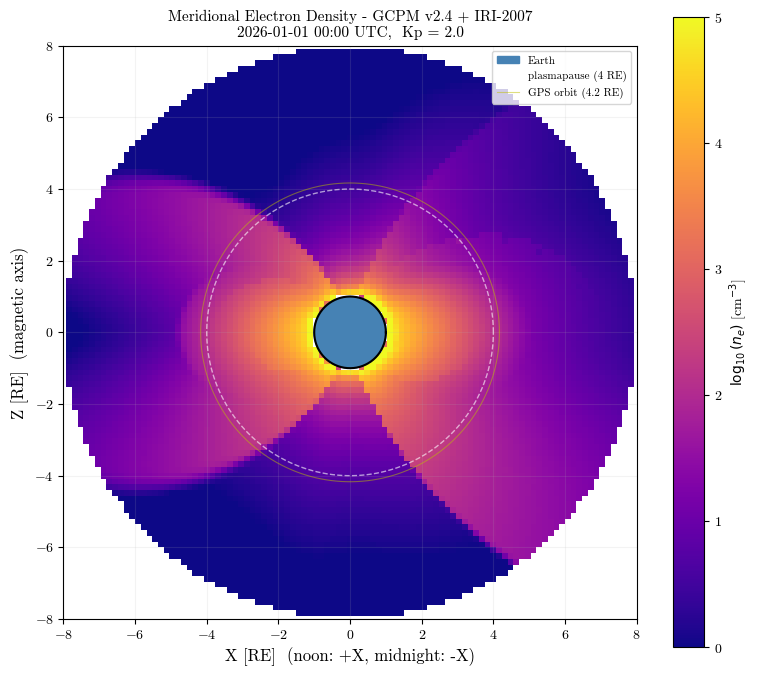
gcpm_v24(dt, r_RE, amlt, alatr, kp) returns electron and ion densities for the requested magnetic coordinates:
r_RE: geocentric distance in Earth radii;amlt: magnetic local time in hours;alatr: magnetic latitude in radians;kp: geomagnetic activity index.
We sample the noon-midnight meridian plane. The resulting plot shows where the dense plasmasphere sits relative to Earth and why link tangent altitude matters.
[3]:
RE_km = plasma.RE  # 6371 km
N = 101
R_MAX = 8.0  # Earth radii

x_RE = np.linspace(-R_MAX, R_MAX, N)  # equatorial radial axis: +X = noon, -X = midnight
z_RE = np.linspace(-R_MAX, R_MAX, N)  # along the magnetic (dipole) axis
XX, ZZ = np.meshgrid(x_RE, z_RE)

ne_grid = np.full((N, N), np.nan)

print(f"Sampling GCPM on {N}x{N} meridional grid (r < {R_MAX} Rₑ)...")
for i in range(N):
    for j in range(N):
        x, z = XX[i, j], ZZ[i, j]
        r = np.hypot(x, z)
        if r < 1.01 or r > R_MAX - 0.01:
            continue
        # magnetic latitude in RADIANS (gcpm_v24 expects radians, matching
        # ex_plasma_meridianal_slice.cc): angle above/below the equatorial plane
        alatr = np.arctan2(z, np.abs(x))
        # noon-midnight meridian: +X side = 12 h (noon), -X side = 0 h (midnight)
        amlt = 12.0 if x >= 0 else 0.0
        ne = plasma.gcpm_v24(dt, r, amlt, alatr, kp)[0]
        if ne > 0:
            ne_grid[i, j] = ne

print("Done.")
ne_valid = ne_grid[np.isfinite(ne_grid)]
print(f"ne range: {ne_valid.min():.2e} – {ne_valid.max():.2e} cm⁻³")
Sampling GCPM on 101x101 meridional grid (r < 8.0 Rₑ)...
Done.
ne range: 1.58e-01 – 1.55e+06 cm⁻³
[4]:
theta_circ = np.linspace(0, 2 * np.pi, 360)

fig, ax = plt.subplots(figsize=(8, 7))

ne_log = np.log10(ne_grid)  # NaN outside domain
im = ax.pcolormesh(XX, ZZ, ne_log, cmap="plasma", vmin=0, vmax=5, shading="auto")
cbar = fig.colorbar(im, ax=ax, label=r"$\log_{10}(n_e)$ [cm$^{-3}$]")

# Earth
ax.fill(
    np.cos(theta_circ), np.sin(theta_circ), color="steelblue", zorder=5, label="Earth"
)
ax.plot(np.cos(theta_circ), np.sin(theta_circ), "k-", lw=1.5, zorder=6)

# Approximate plasmapause at 4 Rₑ
ax.plot(
    4 * np.cos(theta_circ),
    4 * np.sin(theta_circ),
    "w--",
    lw=1.0,
    alpha=0.6,
    label="plasmapause (4 RE)",
)

# GPS MEO orbit
r_gps = 26560 / RE_km
ax.plot(
    r_gps * np.cos(theta_circ),
    r_gps * np.sin(theta_circ),
    "y-",
    lw=0.8,
    alpha=0.5,
    label=f"GPS orbit ({r_gps:.1f} RE)",
)

ax.set_xlabel("X [RE]  (noon: +X, midnight: -X)", fontsize=12)
ax.set_ylabel("Z [RE]  (magnetic axis)", fontsize=12)
ax.set_title(
    f"Meridional Electron Density - GCPM v2.4 + IRI-2007\n"
    f"{YEAR}-{MONTH:02d}-{DAY:02d} {HOUR:02d}:00 UTC,  Kp = {kp:.1f}",
    fontsize=11,
)
ax.set_xlim(-R_MAX, R_MAX)
ax.set_ylim(-R_MAX, R_MAX)
ax.set_aspect("equal")
ax.legend(loc="upper right", fontsize=8)
ax.grid(alpha=0.15)
plt.tight_layout()
plt.show()
Part 2: Ray trace from GPS to a lunar receiver
We propagate a representative GPS satellite and a lunar ELFO receiver, then call trace_ray along their line of sight. The ray tracer integrates the plasma model along the path and returns TEC plus first-, second-, and third-order ionospheric delay terms.
The orbits match Example 5 so the plasma result can be connected directly to the later GNSS measurement simulation.
[5]:
# ── Orbital elements ────────────────────────────────────────────────────────
DEG = np.pi / 180

# GPS satellite in circular MEO (a, e, i, RAAN, omega, M) — all angles in rad.
# GPS orbits the Earth, so its position is already Earth-centred ECI.
#
# The mean anomaly is chosen so the GPS is on the FAR side of the Earth from the
# Moon: only then does the GPS→ELFO line of sight graze the plasmasphere (closest
# approach ~1.6 Rₑ at this epoch). With the ELFO at the Moon (~55 Rₑ), a GPS on
# the same side as the Moon would give a line of sight that never dips below the
# 4 Rₑ cutoff — i.e. no plasma crossing and TEC = 0. (M is tuned for the fixed
# 2026-01-01 epoch; change the epoch and this value must be re-tuned.)
M_GPS_GRAZE = 245.0 * DEG
coe_gps = np.array([26560.0, 0.001, 55.0 * DEG, 0.0, 0.0, M_GPS_GRAZE])
gps_sat = plasma.Satellite(1, coe_gps, epoch_j2000, plasma.GM_EARTH)
pos_tx_km = np.array(gps_sat.get_pos())  # Earth-centred ECI [km]

# ELFO receiver: a=6541.4 km, e=0.6, i=56.2°, ω=90° (frozen).
# The ELFO orbits the MOON, so propagate it with the lunar GM to get a
# MOON-CENTRED inertial position, then shift by the Moon's Earth-relative
# position to express it in the same Earth-centred ECI frame as the GPS Tx and
# the plasma ray-tracer.
# The plasma module works in km³/s² (plasma.GM_EARTH ≈ 398600.44); convert the
# SI pnt.GM_MOON [m³/s²] accordingly.
GM_MOON_km = pnt.GM_MOON / 1e9  # m³/s² -> km³/s²
coe_elfo = np.array([6541.4, 0.6, 56.2 * DEG, 0.0, 90.0 * DEG, np.pi])
elfo_sat = plasma.Satellite(100, coe_elfo, epoch_j2000, GM_MOON_km)
pos_rx_moon_km = np.array(elfo_sat.get_pos())  # Moon-centred inertial [km]

# Moon position relative to Earth in the GCRF (~ECI/J2000) frame.
# get_body_pos returns SI (metres); epoch_j2000 (UTC) ≈ TDB here (the ~69 s
# offset moves the Moon <100 km, negligible against the ~384 000 km distance).
pos_moon_km = (
    np.array(pnt.get_body_pos(epoch_j2000, pnt.EARTH, pnt.MOON, pnt.GCRF)) / 1e3
)

pos_rx_km = pos_rx_moon_km + pos_moon_km  # Earth-centred ECI [km]

r_tx = np.linalg.norm(pos_tx_km)
r_rx = np.linalg.norm(pos_rx_km)
print(f"GPS  position   : {pos_tx_km}  km")
print(f"               |r| = {r_tx:.0f} km = {r_tx/RE_km:.2f} Rₑ")
print(f"Moon position   : {pos_moon_km}  km")
print(
    f"               |r| = {np.linalg.norm(pos_moon_km):.0f} km = {np.linalg.norm(pos_moon_km)/RE_km:.2f} Rₑ"
)
print(
    f"ELFO (Moon-ctr) : {pos_rx_moon_km}  km  (|r| = {np.linalg.norm(pos_rx_moon_km):.0f} km)"
)
print(f"ELFO (Earth-ctr): {pos_rx_km}  km")
print(f"               |r| = {r_rx:.0f} km = {r_rx/RE_km:.2f} Rₑ")
GPS  position   : [-11273.10341725 -13801.0200303  -19709.89924729]  km
               |r| = 26571 km = 4.17 Rₑ
Moon position   : [144298.61281474 289594.52147969 160163.5805565 ]  km
               |r| = 361026 km = 56.67 Rₑ
ELFO (Moon-ctr) : [-1.28174473e-12 -5.82232342e+03 -8.69728289e+03]  km  (|r| = 10466 km)
ELFO (Earth-ctr): [144298.61281474 283772.19805692 151466.2976648 ]  km
               |r| = 352549 km = 55.34 Rₑ
[6]:
# ── RayTraceConfig ──────────────────────────────────────────────────────────
# Cutoff: only model plasma below 4 Rₑ; above that the medium is vacuum.
CUTOFF_RE = 4.0

config = plasma.RayTraceConfig()
config.freq_Hz = plasma.freq_L1  # 1575.42 MHz
config.step_size = 100.0  # integration step [km]
config.correction = True  # apply receiver-position correction
config.fine_correction = False  # skip iterative fine correction
config.correction_method = "neldermead"  # solver for position correction
config.cutoff_r = CUTOFF_RE * RE_km
config.kp = kp
config.gradn_dx = 1.0  # refractive-index gradient step [km]
config.integ_method = "rk4"
config.use_fortran_gcpm = False
config.straight_ray = False

print(f"Frequency   : {config.freq_Hz*1e-6:.3f} MHz  (L1)")
print(f"Step size   : {config.step_size:.0f} km")
print(f"Cutoff      : {CUTOFF_RE} Rₑ = {config.cutoff_r:.0f} km")
print(f"Kp          : {config.kp:.2f}")
Frequency   : 1575.420 MHz  (L1)
Step size   : 100 km
Cutoff      : 4.0 Rₑ = 25484 km
Kp          : 2.00
[7]:
print("Running ray-trace (correction=True, fine_correction=False) ...")
pp = plasma.trace_ray(
    epoch_j2000, pos_tx_km, pos_rx_km, config, debug_prop=False, debug_corr=False
)

print()
print("=== Ray-Trace Results ===")
print(f"  TEC (total)      : {pp.tecu:.3f} TECU")
print(f"  L1 total delay   : {pp.total_delay_m:.4f} m")
print(f"    TEC delay      : {pp.tec_delay_m:.4f} m")
print(f"    Bending delay  : {pp.dist_bend_m:.6f} m")
print(f"  Straight dist    : {pp.dist_straight_km:.1f} km")
Running ray-trace (correction=True, fine_correction=False) ...

=== Ray-Trace Results ===
  TEC (total)      : 4.969 TECU
  L1 total delay   : 0.8068 m
    TEC delay      : 0.8069 m
    Bending delay  : 0.000001 m
  Straight dist    : 376900.1 km
[8]:
# ── Visualise ray path and density profile ───────────────────────────────────
pos_path = np.array(pp.pos_eci)  # [N_steps x 3] km, ECI (covers the plasma leg)
r_path = np.array(pp.r)  # geocentric distance [km]
s_path = np.array(pp.s)  # arc length [km]

alt_path = r_path - RE_km  # altitude [km]

# Electron density along path (re-compute cheaply at each step)
ne_path = np.array(
    [plasma.compute_ne(epoch_j2000, pos_path[k], config) for k in range(len(s_path))]
)

# Only the segment inside the 4 Rₑ cutoff carries plasma; truncate the profile
# plots there (everything beyond is vacuum out to the Moon). "up to the 4 Rₑ
# crossing" = up to the last sample still within the cutoff radius.
in_plasma = r_path <= config.cutoff_r
k_end = np.max(np.nonzero(in_plasma)) + 1 if in_plasma.any() else len(r_path)
sl = slice(0, k_end)
k_peri = int(np.argmin(r_path[sl]))  # perigee (densest) index

fig, axes = plt.subplots(1, 3, figsize=(15, 5))

# --- Plot A: ray path in XZ plane (near-Earth plasma region) ----------------
ax = axes[0]
sc = ax.scatter(
    pos_path[sl, 0] / RE_km,
    pos_path[sl, 2] / RE_km,
    c=np.log10(np.where(ne_path[sl] > 0, ne_path[sl], np.nan)),
    cmap="plasma",
    s=8,
    vmin=0,
    vmax=4,
    zorder=4,
)
fig.colorbar(sc, ax=ax, label=r"$\log_{10}(n_e)$ [cm$^{-3}$]", shrink=0.8)
ax.scatter(
    *pos_tx_km[[0, 2]] / RE_km,
    marker="*",
    s=250,
    color="gold",
    zorder=10,
    label="GPS Tx",
)
# Earth
ax.fill(np.cos(theta_circ), np.sin(theta_circ), color="steelblue", zorder=5)
ax.plot(np.cos(theta_circ), np.sin(theta_circ), "k-", lw=1.5, zorder=6)
ax.plot(
    CUTOFF_RE * np.cos(theta_circ),
    CUTOFF_RE * np.sin(theta_circ),
    "k--",
    lw=0.8,
    alpha=0.5,
    label=f"cutoff ({CUTOFF_RE} Rₑ)",
)
# Direction to the Moon / ELFO Rx (it sits ~55 Rₑ away, off-plot)
moon_dir = pos_moon_km[[0, 2]] / np.linalg.norm(pos_moon_km[[0, 2]])
ax.annotate(
    "to Moon / ELFO Rx",
    xy=moon_dir * 4.6,
    xytext=moon_dir * 2.6,
    fontsize=8,
    ha="center",
    va="center",
    arrowprops=dict(arrowstyle="->", color="cyan", lw=1.5),
)
LIM = 5.0
ax.set_xlim(-LIM, LIM)
ax.set_ylim(-LIM, LIM)
ax.set_xlabel("X [Rₑ]")
ax.set_ylabel("Z [Rₑ]")
ax.set_title("Ray Path through Plasmasphere (XZ plane)\n(coloured by $n_e$)")
ax.legend(fontsize=8, loc="lower left")
ax.set_aspect("equal")
ax.grid(alpha=0.2)

# --- Plot B: altitude profile (to the 4 Rₑ crossing) ------------------------
ax2 = axes[1]
ax2.plot(s_path[sl], alt_path[sl], "b-", lw=1.5)
ax2.scatter(
    s_path[sl][k_peri],
    alt_path[sl][k_peri],
    color="b",
    zorder=5,
    label=f"perigee ({alt_path[sl][k_peri]:.0f} km)",
)
ax2.axhline(
    (CUTOFF_RE - 1) * RE_km,
    color="gray",
    lw=0.8,
    ls=":",
    label=f"cutoff {CUTOFF_RE} Rₑ",
)
ax2.set_xlabel("Arc length along ray [km]")
ax2.set_ylabel("Altitude [km]")
ax2.set_title("Altitude Profile (to 4 Rₑ crossing)")
ax2.legend(fontsize=8)
ax2.grid(alpha=0.3)

# --- Plot C: electron density profile (to the 4 Rₑ crossing) ----------------
ax3 = axes[2]
ne_plot = np.where(ne_path[sl] > 0, ne_path[sl], np.nan)
ax3.semilogy(s_path[sl], ne_plot, "r-", lw=1.5)
ax3.scatter(
    s_path[sl][k_peri],
    ne_plot[k_peri],
    color="r",
    zorder=5,
    label=f"peak ≈ {np.nanmax(ne_plot):.0f} cm⁻³",
)
ax3.set_xlabel("Arc length along ray [km]")
ax3.set_ylabel(r"$n_e$ [cm$^{-3}$]")
ax3.set_title("Electron Density (to 4 Rₑ crossing)")
ax3.legend(fontsize=8)
ax3.grid(alpha=0.3, which="both")

fig.suptitle(
    f"GPS → ELFO Ray-Trace  |  L1  |  Kp={kp:.1f}  |  "
    f"TEC = {pp.tecu:.2f} TECU  |  L1 delay = {pp.total_delay_m:.3f} m",
    fontsize=11,
    y=1.01,
)
plt.tight_layout()
plt.show()
/var/folders/1f/_8g3y5td38n93nph4z3c5d4c0000gn/T/ipykernel_73950/2983830663.py:122: UserWarning: Glyph 8337 (\N{LATIN SUBSCRIPT SMALL LETTER E}) missing from font(s) cmr10.
  plt.tight_layout()
/var/folders/1f/_8g3y5td38n93nph4z3c5d4c0000gn/T/ipykernel_73950/2983830663.py:122: UserWarning: Glyph 8776 (\N{ALMOST EQUAL TO}) missing from font(s) cmr10.
  plt.tight_layout()
/var/folders/1f/_8g3y5td38n93nph4z3c5d4c0000gn/T/ipykernel_73950/2983830663.py:122: UserWarning: Glyph 8315 (\N{SUPERSCRIPT MINUS}) missing from font(s) cmr10.
  plt.tight_layout()
/var/folders/1f/_8g3y5td38n93nph4z3c5d4c0000gn/T/ipykernel_73950/2983830663.py:122: UserWarning: Glyph 8594 (\N{RIGHTWARDS ARROW}) missing from font(s) cmr10.
  plt.tight_layout()
/Users/keidaiiiyama/Documents/sw_navlab/LuPNT/.pixi/envs/default/lib/python3.11/site-packages/IPython/core/pylabtools.py:170: UserWarning: Glyph 8337 (\N{LATIN SUBSCRIPT SMALL LETTER E}) missing from font(s) cmr10.
  fig.canvas.print_figure(bytes_io, **kw)
/Users/keidaiiiyama/Documents/sw_navlab/LuPNT/.pixi/envs/default/lib/python3.11/site-packages/IPython/core/pylabtools.py:170: UserWarning: Glyph 8776 (\N{ALMOST EQUAL TO}) missing from font(s) cmr10.
  fig.canvas.print_figure(bytes_io, **kw)
/Users/keidaiiiyama/Documents/sw_navlab/LuPNT/.pixi/envs/default/lib/python3.11/site-packages/IPython/core/pylabtools.py:170: UserWarning: Glyph 8315 (\N{SUPERSCRIPT MINUS}) missing from font(s) cmr10.
  fig.canvas.print_figure(bytes_io, **kw)
/Users/keidaiiiyama/Documents/sw_navlab/LuPNT/.pixi/envs/default/lib/python3.11/site-packages/IPython/core/pylabtools.py:170: UserWarning: Glyph 8594 (\N{RIGHTWARDS ARROW}) missing from font(s) cmr10.
  fig.canvas.print_figure(bytes_io, **kw)
Why the density profile (Plot C) looks like it has a “jump”
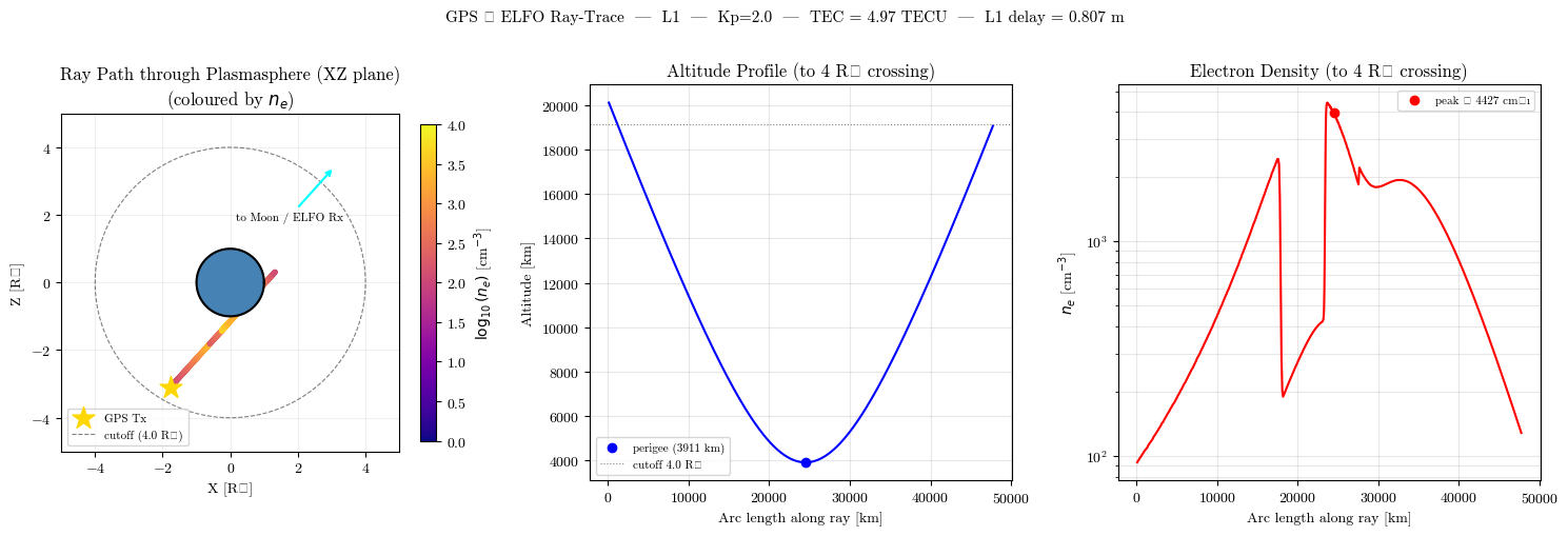
The \(n_e\) curve shows two near-vertical walls (a steep drop on the inbound leg and a steep rise back up toward perigee). These are not a discontinuity or a bug — they are the real, steep-but-continuous gradient across the plasmapause / inner-plasmasphere boundary of the GCPM v2.4 model.
Two things make a smooth gradient look like a step here:
The arc-length axis is compressed. The plotted path spans ~0–50 000 km, but each transition is only ~200–400 km wide. On a log-\(n_e\) axis, a factor-of-$:nbsphinx-math:`sim`$10 change over a few hundred km is thinner than a plot pixel, so it renders as a vertical cliff.
The integration step is coarse. With
config.step_size = 100 km, only 2–4 samples land inside each transition, connecting the top and bottom with what looks like a single vertical segment.
Resampling the exact same path finely (2 km) shows the walls are in fact smooth and monotonic: e.g. across the inbound wall \(n_e\) falls from ~2000 to ~330 cm⁻³ over ~230 km, and across the perigee-side wall it rises from ~450 to ~4400 cm⁻³ over ~450 km — no jump, no NaN, no sign flip.
The steepness is physical: in compute_ne the receiver position is converted to solar-magnetic coordinates with a continuous magnetic local time (unlike the hard noon/midnight amlt switch used only for the Part 1 grid), and every GCPM region boundary (plasmapause, inner-plasmasphere bridge, trough, IRI bridge, polar cap) is blended with a smooth switchon() transition — so the field is continuous by construction, just sharp near the plasmapause. The density peak sitting slightly
off the geometric perigee is the same effect: the plasma is organized by dipole L-shell and magnetic latitude, not by geocentric radius.
To render it smoothly, reduce config.step_size (e.g. to 25 km, at higher compute cost) or zoom the arc-length axis onto the near-Earth plasma leg.