Example 17: Satellite-to-Satellite Angles-Only OD — authored in Python
A minimal orbit-determination scenario built entirely in Python — the estimator application and the measurement model are Python classes, driven by the same C++ pnt.Simulation as every other example. This is the template for prototyping your own scenario without touching C++.
Two Spacecraft share the lunar environment. An observer measures only the bearing (unit line-of-sight direction) to a target whose ephemeris is treated as known, and an EKF on the observer estimates the observer’s own 6-state orbit \([\mathbf r,\mathbf v]\) (no clock — angles are clock-independent). Measuring a direction to a known landmark is well-posed and converges; estimating an unknown target’s range from bearings alone is the classic ill-posed angles-only
problem, and is not attempted.
The pieces (see the How to Create a New Simulation page → “Working in Python”):
a Measurement — subclass
pnt.Measurement, implementcompute(self, x) -> (z, H, R);an Application — subclass
pnt.Application(an EKF in numpy), registered withpnt.register_applicationand referenced byclass:inconfigs/sat_bearing_odts.yaml;reused as-is: the
Spacecraftagents, thepnt.NBodyDynamicsforce model (built and propagated with STM from Python), and Monte-Carlo (looped here over seeds).
[1]:
import os, sys
from pathlib import Path
import numpy as np
import matplotlib.pyplot as plt

for _base in [Path.cwd(), *Path.cwd().parents]:
    if (_base / "python" / "pylupnt" / "__init__.py").exists():
        sys.path.insert(0, str((_base / "python").resolve()))
        if (_base / "data" / "LuPNT_data").is_dir():
            os.environ["LUPNT_DATA_PATH"] = str((_base / "data" / "LuPNT_data").resolve())
        break
import yaml
import pylupnt as pnt
print(f"pylupnt loaded from: {pnt.__file__}")
[00.01][PyLuPNT] Initializing
pylupnt loaded from: /Users/keidaiiiyama/Documents/sw_navlab/LuPNT/python/pylupnt/__init__.py
1. Author the measurement model in Python
A pnt.Measurement subclass returns the predicted observable \(z=h(x)\), its Jacobian \(H=\partial h/\partial x\), and the noise covariance \(R\). m.evaluate(x) runs it through the C++ base (the same path a filter uses), so the same class both generates an observation (apply to a truth state, add noise) and predicts one (apply to the filter state).
[2]:
class BearingMeasurement(pnt.Measurement):
    "Unit line-of-sight (bearing) to a known target position."
    def __init__(self, sigma_rad):
        pnt.Measurement.__init__(self)
        self.sigma = sigma_rad
        self.target = np.zeros(3)          # set per-epoch to the target truth position

    def compute(self, x):                  # -> (z = h(x), H = dh/dx, R)
        d = self.target - x[:3]; rn = np.linalg.norm(d); u = d / rn
        H = np.zeros((3, 6)); H[:, :3] = -(np.eye(3) - np.outer(u, u)) / rn
        return u, H, self.sigma**2 * np.eye(3)
2. Author the estimator application in Python
A pnt.Application subclass. setup() builds a filter force model (pnt.NBodyDynamics) and the measurement; step(t) reads truth through the host agent, runs one EKF predict/update (propagating with STM via dyn.propagate_stm), and stores results on self. The engine constructs it from the application: block of the config and calls step each epoch.
[3]:
def make_dyn():
    d = pnt.NBodyDynamics()
    for b in (pnt.Body.Moon(8, 8), pnt.Body.Earth(), pnt.Body.Sun()):
        d.add_body(b)
    d.set_frame(pnt.Frame.MOON_CI); d.set_integrator(pnt.IntegratorType.RKF45); d.set_autodiff(True)
    return d


class PyAnglesOdtsApp(pnt.Application):
    def __init__(self, config):
        pnt.Application.__init__(self)
        self.target = config["target"]
        self.set_frequency(config.get("frequency", 1.0 / 60))
        self.sigma = np.radians(config.get("angle_sigma_arcsec", 2.0) / 3600.0)
        self.p0 = config.get("initial_position_sigma_m", 300.0)
        self.v0 = config.get("initial_velocity_sigma_mps", 0.3)
        self.qa = config.get("process_accel_sigma_mps2", 1e-6)
        self.rng = np.random.default_rng(config.get("seed", 42))
        self.times, self.est, self.truth, self.sig = [], [], [], []
        self._init = False

    def setup(self):
        pnt.Application.setup(self)             # base schedules step() at get_frequency()
        self.dyn = make_dyn()
        self.meas = BearingMeasurement(self.sigma)

    def step(self, t):
        if not self._init:                      # capture initial truths once
            self.obs = np.asarray(self.get_agent().get_state_at(0.0))
            self.tgt = np.asarray(self.get_agent().get_world().get_state_at(self.target, 0.0))
            self.x = self.obs + np.r_[self.rng.normal(0, self.p0, 3), self.rng.normal(0, self.v0, 3)]
            self.P = np.diag(np.r_[[self.p0**2]*3, [self.v0**2]*3])
            self._init, self._t = True, t
            self._log(t); return
        dt = t - self._t
        self.obs = np.asarray(self.dyn.propagate_stm(self.obs, float(self._t), float(t))[0]).ravel()
        self.tgt = np.asarray(self.dyn.propagate_stm(self.tgt, float(self._t), float(t))[0]).ravel()
        xf, F = self.dyn.propagate_stm(self.x, float(self._t), float(t))
        self.x = np.asarray(xf).ravel(); F = np.asarray(F); self._t = t
        q = self.qa**2
        Q = q * np.block([[dt**3 / 3 * np.eye(3), dt**2 / 2 * np.eye(3)],
                          [dt**2 / 2 * np.eye(3), dt * np.eye(3)]])
        self.P = F @ self.P @ F.T + Q
        self.meas.target = self.tgt[:3]
        z = self.meas.evaluate(self.obs)[0] + self.rng.normal(0, self.sigma, 3)   # generate
        u, H, R = self.meas.evaluate(self.x)                                       # predict
        S = H @ self.P @ H.T + R
        K = self.P @ H.T @ np.linalg.inv(S)
        self.x = self.x + K @ (z - u)
        IKH = np.eye(6) - K @ H
        self.P = IKH @ self.P @ IKH.T + K @ R @ K.T
        self._log(t)

    def _log(self, t):
        self.times.append(t); self.est.append(self.x.copy())
        self.truth.append(self.obs.copy()); self.sig.append(np.sqrt(np.diag(self.P)))
3. Register and run
Register the Python app, then hand the scenario config to pnt.Simulation. We run a small Monte-Carlo by looping the seed (each run is a couple of seconds), collecting one ensemble of observer position errors.
[4]:
pnt.register_application("PyAnglesOdtsApp", PyAnglesOdtsApp)

cfg_path = next(p / "configs" / "sat_bearing_odts.yaml"
                for p in [Path.cwd(), *Path.cwd().parents]
                if (p / "configs" / "sat_bearing_odts.yaml").exists())
base_cfg = yaml.safe_load(open(cfg_path))

N_MC = 5
runs = []
for i in range(N_MC):
    cfg = yaml.safe_load(open(cfg_path))
    cfg["agents"]["observer"]["application"]["seed"] = 42 + i
    sim = pnt.Simulation(cfg); sim.run()
    runs.append(sim.get_agent("observer").get_application())

r0 = runs[0]
t_hr = np.asarray(r0.times) / 3600.0
perr = np.array([np.linalg.norm(np.array(r.est)[:, :3] - np.array(r.truth)[:, :3], axis=1)
                 for r in runs])            # [N_MC, N]
print(f"{N_MC} Monte-Carlo runs")
print(f"Final observer position error (RMS over MC): {np.sqrt(np.mean(perr[:, -1]**2)):8.2f} m")
print(f"Arc   observer position error (RMS over MC): {np.sqrt(np.mean(perr**2)):8.2f} m")
[01.90][/Users/keidaiiiyama/Documents/sw_navlab/LuPNT/data/LuPNT_data/output/sat_bearing_odts/sat_bearing_odts.h5] Output file: {}
[01.90][Simulation] Output file: /Users/keidaiiiyama/Documents/sw_navlab/LuPNT/data/LuPNT_data/output/sat_bearing_odts/sat_bearing_odts.h5

  0%|          | 0/100 [00:00<00:00, 0.0 it/s]
[02.11][Simulation]   0%|          | 0/100 [00:00<00:00, 0.0 it/s]
[02.11][Simulation]  13%|█         | 13/100 [00:00<00:01, 64.8 it/s]
[02.11][Simulation]  26%|██        | 26/100 [00:00<00:01, 64.4 it/s]
[02.11][Simulation]  40%|████      | 40/100 [00:00<00:00, 66.2 it/s]
[02.11][Simulation]  54%|█████     | 54/100 [00:00<00:00, 66.9 it/s]
[02.11][Simulation]  68%|██████    | 68/100 [00:01<00:00, 67.5 it/s]
[02.11][Simulation]  81%|████████  | 81/100 [00:01<00:00, 66.9 it/s]
[02.11][Simulation]  95%|█████████ | 95/100 [00:01<00:00, 67.2 it/s]
[02.11][Simulation] 100%|██████████| 100/100 [00:01<00:00, 67.8 it/s]
[02.11][Simulation] 100%|██████████| 100/100 [00:01<00:00, 67.7 it/s]
[02.11][Simulation] 100%|██████████| 100/100 [00:01<00:00, 67.7 it/s]
[02.11][Simulation] 100%|██████████| 100/100 [00:01<00:00, 67.7 it/s]

  0%|          | 0/100 [00:00<00:00, 0.0 it/s]
[03.62][Simulation]   0%|          | 0/100 [00:00<00:00, 0.0 it/s]
[03.62][Simulation]  13%|█         | 13/100 [00:00<00:01, 64.5 it/s]
[03.62][Simulation]  27%|██        | 27/100 [00:00<00:01, 66.6 it/s]
[03.62][Simulation]  40%|████      | 40/100 [00:00<00:00, 65.7 it/s]
[03.62][Simulation]  54%|█████     | 54/100 [00:00<00:00, 66.6 it/s]
[03.62][Simulation]  68%|██████    | 68/100 [00:01<00:00, 67.1 it/s]
[03.62][Simulation]  81%|████████  | 81/100 [00:01<00:00, 66.6 it/s]
[03.62][Simulation]  95%|█████████ | 95/100 [00:01<00:00, 66.9 it/s]
[03.62][Simulation] 100%|██████████| 100/100 [00:01<00:00, 67.3 it/s]
[03.62][Simulation] 100%|██████████| 100/100 [00:01<00:00, 67.2 it/s]
[03.62][Simulation] 100%|██████████| 100/100 [00:01<00:00, 67.2 it/s]
[03.62][Simulation] 100%|██████████| 100/100 [00:01<00:00, 67.2 it/s]

  0%|          | 0/100 [00:00<00:00, 0.0 it/s]
[05.13][Simulation]   0%|          | 0/100 [00:00<00:00, 0.0 it/s]
[05.13][Simulation]  13%|█         | 13/100 [00:00<00:01, 64.9 it/s]
[05.13][Simulation]  26%|██        | 26/100 [00:00<00:01, 64.5 it/s]
[05.13][Simulation]  40%|████      | 40/100 [00:00<00:00, 66.3 it/s]
[05.13][Simulation]  53%|█████     | 53/100 [00:00<00:00, 65.9 it/s]
[05.13][Simulation]  67%|██████    | 67/100 [00:01<00:00, 66.7 it/s]
[05.13][Simulation]  81%|████████  | 81/100 [00:01<00:00, 67.2 it/s]
[05.13][Simulation]  94%|█████████ | 94/100 [00:01<00:00, 66.8 it/s]
[05.13][Simulation] 100%|██████████| 100/100 [00:01<00:00, 67.3 it/s]
[05.13][Simulation] 100%|██████████| 100/100 [00:01<00:00, 67.2 it/s]
[05.13][Simulation] 100%|██████████| 100/100 [00:01<00:00, 67.2 it/s]
[05.13][Simulation] 100%|██████████| 100/100 [00:01<00:00, 67.2 it/s]

  0%|          | 0/100 [00:00<00:00, 0.0 it/s]
[06.65][Simulation]   0%|          | 0/100 [00:00<00:00, 0.0 it/s]
[06.65][Simulation]  13%|█         | 13/100 [00:00<00:01, 64.7 it/s]
[06.65][Simulation]  26%|██        | 26/100 [00:00<00:01, 64.7 it/s]
[06.65][Simulation]  40%|████      | 40/100 [00:00<00:00, 66.2 it/s]
[06.65][Simulation]  54%|█████     | 54/100 [00:00<00:00, 67.0 it/s]
[06.65][Simulation]  68%|██████    | 68/100 [00:01<00:00, 67.5 it/s]
[06.65][Simulation]  81%|████████  | 81/100 [00:01<00:00, 67.0 it/s]
[06.65][Simulation]  93%|█████████ | 93/100 [00:01<00:00, 65.8 it/s]
[06.65][Simulation] 100%|██████████| 100/100 [00:01<00:00, 66.6 it/s]
[06.65][Simulation] 100%|██████████| 100/100 [00:01<00:00, 66.6 it/s]
[06.65][Simulation] 100%|██████████| 100/100 [00:01<00:00, 66.5 it/s]
[06.65][Simulation] 100%|██████████| 100/100 [00:01<00:00, 66.5 it/s]

  0%|          | 0/100 [00:00<00:00, 0.0 it/s]
[08.18][Simulation]   0%|          | 0/100 [00:00<00:00, 0.0 it/s]
[08.18][Simulation]  13%|█         | 13/100 [00:00<00:01, 64.2 it/s]
[08.18][Simulation]  27%|██        | 27/100 [00:00<00:01, 67.0 it/s]
[08.18][Simulation]  40%|████      | 40/100 [00:00<00:00, 66.0 it/s]
[08.18][Simulation]  54%|█████     | 54/100 [00:00<00:00, 66.8 it/s]
[08.18][Simulation]  68%|██████    | 68/100 [00:01<00:00, 67.3 it/s]
[08.18][Simulation]  81%|████████  | 81/100 [00:01<00:00, 66.8 it/s]
[08.18][Simulation]  95%|█████████ | 95/100 [00:01<00:00, 67.3 it/s]
[08.18][Simulation] 100%|██████████| 100/100 [00:01<00:00, 67.4 it/s]
[08.18][Simulation] 100%|██████████| 100/100 [00:01<00:00, 67.4 it/s]
[08.18][Simulation] 100%|██████████| 100/100 [00:01<00:00, 67.4 it/s]
[08.18][Simulation] 100%|██████████| 100/100 [00:01<00:00, 67.4 it/s]
5 Monte-Carlo runs
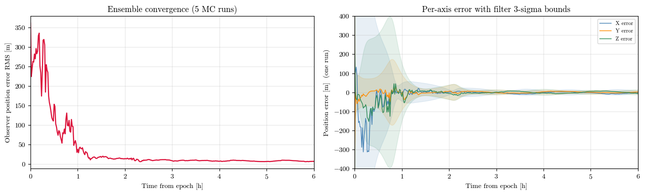
Final observer position error (RMS over MC):     6.31 m
Arc   observer position error (RMS over MC):    76.84 m
4. Convergence
Left: the ensemble position-error RMS (over the Monte-Carlo runs) — from the ~300 m a-priori down to the metre level as the bearing geometry accumulates. Right: the per-axis error of one run with the filter’s own \(3\sigma\) envelope (the estimate stays inside its covariance).
[5]:
fig, (ax0, ax1) = plt.subplots(1, 2, figsize=(13, 4))
ax0.plot(t_hr, np.sqrt(np.mean(perr**2, axis=0)), color="crimson", lw=1.6)
ax0.set_xlabel("Time from epoch [h]"); ax0.set_ylabel("Observer position error RMS [m]")
ax0.set_title(f"Ensemble convergence ({N_MC} MC runs)")
ax0.set_xlim(0, t_hr[-1]); ax0.grid(True, alpha=0.3)

est = np.array(r0.est); truth = np.array(r0.truth); sig = np.array(r0.sig)
err = est - truth
for k, (lab, col) in enumerate(zip("XYZ", ["steelblue", "darkorange", "seagreen"])):
    ax1.plot(t_hr, err[:, k], color=col, lw=1.0, label=f"{lab} error")
    ax1.fill_between(t_hr, -3 * sig[:, k], 3 * sig[:, k], color=col, alpha=0.12)
ax1.set_xlabel("Time from epoch [h]"); ax1.set_ylabel("Position error [m]  (one run)")
ax1.set_title("Per-axis error with filter 3-sigma bounds")
ax1.set_xlim(0, t_hr[-1]); ax1.set_ylim(-400, 400)
ax1.legend(fontsize=8, loc="upper right"); ax1.grid(True, alpha=0.3)
plt.tight_layout(); plt.show()
5. Observer orbit
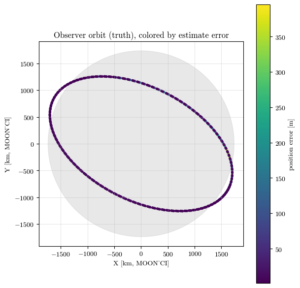
The observer’s true trajectory (Moon-centered inertial, X–Y projection) colored by the estimate error magnitude — the Python-authored EKF recovers the orbit to the metre level.
[6]:
fig, ax = plt.subplots(figsize=(6.2, 6))
R_MOON_KM = 1737.4
th = np.linspace(0, 2 * np.pi, 200)
ax.fill(R_MOON_KM * np.cos(th), R_MOON_KM * np.sin(th), color="lightgray", alpha=0.5)
en = np.linalg.norm(est[:, :3] - truth[:, :3], axis=1)
sc = ax.scatter(truth[:, 0] / 1e3, truth[:, 1] / 1e3, c=en, cmap="viridis", s=8)
ax.set_aspect("equal"); ax.set_xlabel("X [km, MOON_CI]"); ax.set_ylabel("Y [km, MOON_CI]")
ax.set_title("Observer orbit (truth), colored by estimate error")
plt.colorbar(sc, ax=ax, label="position error [m]"); ax.grid(True, alpha=0.3)
plt.tight_layout(); plt.show()
Summary
A complete OD scenario — the estimator Application and the Measurement model — authored in pure Python, driven by the C++
pnt.Simulation(pnt.register_application+configs/sat_bearing_odts.yaml).The filter reuses
pnt.NBodyDynamics(built and propagated with STM from Python) and theSpacecraftagents; only new observables and estimators are written, and here in Python.Angles-only navigation against a known landmark is observable and converges (a few metres over a 6 h arc from a 300 m a-priori with 2 arcsec bearings).
This is the smallest template for authoring your own scenario in Python — see How to Create a New Simulation → “Working in Python” for
pnt.Agentand more.